UNIVERSAL
ROBOTS

For model UR-6-85-5-A
Training Manual.
Hint and tips Version 1.4
March 2012.
Zacobria Pte. Ltd.
This manual provides some in depth and step by
step introduction and use of the Universal-Robots. After reading this manual
you will be able to use and program the Universal-Robot (UR).
Aside from this manual there is the original
UR user manual (manual_enx.x.pdf) wish also is very good and provide other
detailed information’s for using the UR and it is recommended to read both
manuals. Especially the reading the safety section and risk assessment is necessary
to read before going any further.
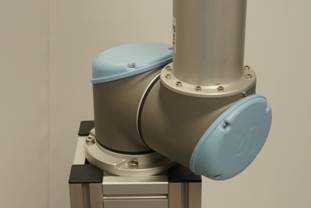
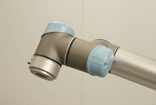
The UR is a very innovative and user friendly
product and it is also interesting to know a little about the inside of the
robot – especially when the covers are so easy to remove which can be done
without any harm - however just look – don’t touch anything inside the joint or
even turn any screws inside because the encoder can then get out of adjustment
and the robot will malfunction and the warranty is void – so just close the lid
again – see also photo at the end of this manual of open joint.
One thing you
will experience very fast is that it seems that the robot has its own mind –
which is also true but it is the mind of the programming team who made this
robot, but they did a very good job.
For example when
two far away waypoints has been made then the robot will take a mathematically
and physically possible shortest way from point A to point B – which is maybe
not always what you expected. To control the path – you need more waypoints in
between to force the robot to go through.
The shortest way is also correct in most
cases, but not always the case. Because the movement can be influenced by the
position of the joint. The joints can turn +360 degrees and -360 degrees if the
joint is in its zero position as seen on the move screen (i.e. total 720 degrees).
So how the robot move to next waypoint can be dependent on this.
One way to explain this is - Consider the
joint happen to be in the zero position at beginning of programming and if you
have made several waypoints by only turning the base joint in only one
direction e.g. left so point A = 0 degree, point B = 45 degree, point C = 90
degree, point D = 135 degree - and so on all the way up to 359 degree.
Now you want a
point that is actually at position 361 degree – it is possible to make and
continue programming - BUT when you run the program the robot will start nicely
to turn around as you expected, but when moving from 359 degrees to 361 degrees
it will swing all the way back and go to degree 1 – (always keep a hand on the
E-stop when test running).
This is because
the joints can turn +/-360 degrees.
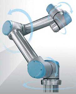
The UR robot is a 6 axis robot which means it
can go to almost any position within each reach except directly above or directly
below where it is sitting itself.
But it also has to be taken into account how
the robot physical are constructed especially the length or the arms and joints.
So just like a human body we might need to change our posture to grab something
with our hand – so do the robot sometimes need to be re position by the
programmer in order to reach the target. You might read the section about
“Singularity” at the end of the manual.
5.1 Turn
on the robot for the second time.
6 Menus
and finding your way around.
8 Move
screen - The Home Position.
8.1 Move
screen - Moving the joints individually.
8.2 Move
screen - move the robot linearly.
8.3 Move
screen - move robot in relation to tool head position.
8.4 Move
screen - Speed regulator.
8.6 Move
screen - X, Y, Z indicator.
8.7 Move
screen - simulator view.
12 Start
programming Lesson 1.
12.2 Programming
- First Program – MoveJ (Non Linear Movements).
12.2.2 Program
“Home” position.
13.1 Programming
- Speed regulator during program run.
13.2 Programming
- Save the file.
14 Programming
- Load a program from USB drive.
14.1 Program
environment tools and indicator.
14.3 MoveL
(Linear movements).
14.4 Singularity
during MoveL.
15 Programming
– Lesson 2 – Inputs and Outputs.
15.1 Reading
Inputs and Setting Outputs.
16 Programming
– Lesson 3 – IF conditions.
16.1 Check
expression continuously
17 Combinations
of expressions:
18 Programming
– Lesson 4 – Special conditions.
19 Programming
– Lesson 5 - Files.
20 Programming
– Lesson 6 - Templates.
21 Programming
– Lesson 7 – Before Start Sequence.
22 Programming
– Lesson 8 – Variables.
22.2 Variables
– Prefer to keep value from last run.
23 Programming
– Lesson 9 – Thread.
23.1 Placing
the work pieces in rows on the conveyor.
23.2 Variables
– Prefer to keep value from last run.
24 Programming
– Lesson 10 - Advanced – Script Programming.
24.1 Script
programming from the teaching pendant.
24.2 Script
program by Socket connection - Host computer to UR robot #1.
24.3 Script
program for Socket connection - Host computer to UR robot #2.
25 Installation
- Features screen:
26 Hardware
– Tool head Digital Outputs are Open collector type:
27 Potential
Free interface with other equipment.
28 Extension
of I/O interfaces by MODBUS nodes.
30 Force
feed back and Safety stop.
32 Connection
of External Emergency stop.
The UR arrives in two similar cardboard boxes
– one with the controller and one with the robot itself. Unpack both boxes and
place the controller on a table or the floor.
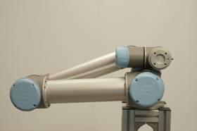
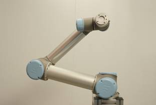
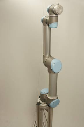
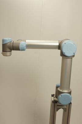
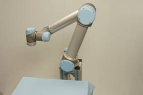
The robot is folded in foetus position and can
be placed on a table, stand or any place that is prepared with 4 holes that fit
the foot base. Since the robot is folded in this transportation position is not
possible right now to fit all 4 bolts, but 1 or two is enough to hold the robot
– so just fit the bolts where the base holes are accessible.
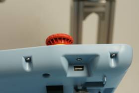
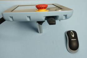
The monitor is a
touch screen monitor and can be operated as it is with pressing the screen and
onscreen keyboard. It is possible to connect a mouse and keyboard to the USB
connector on the side of the monitor and especially a mouse is useful.
Although it is
possible to store your user programs on the internal hard drive (Flash card in
this case) I will recommend to dedicate a small USB thumb drive for your user
programs.
Because they are
then very easy to carry over to your office computer for documentation and
backup purpose and it becomes much easier to version control your programs. To
save on the hard drive and on the USB drive will often lead to confusion for
which is my correct and latest program?
And to copy from
the hard drive over to an office computer is tricky, but using a USB drive
makes its very easy and convenient.
Free USB port. Prepare
an empty USB drive
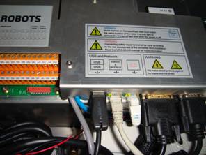
Insert
the USB drive in.
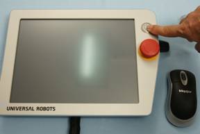
Turn on the power by pressing the ON button on
the monitor.

A messages appears that say “No
Cable” –
Which normal and no action is need
for this.
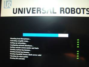
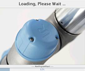
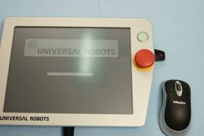
During boot you will see various screens loading and
checks – this is normal and it takes 1 – 2 minutes to boot. You will also hear
the fans turn in the controller box.
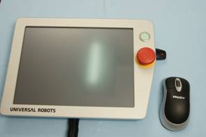
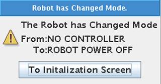
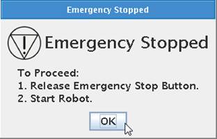
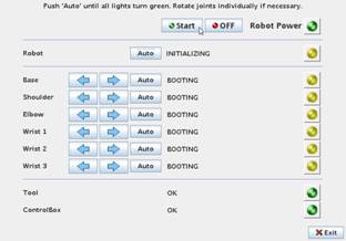
After booting the monitor will show one
of these two screens depending on if the Emergency push button has been
pressed.
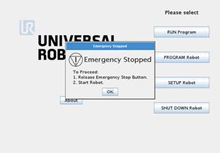
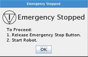
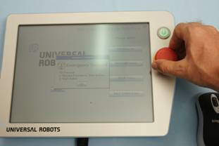
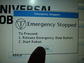
If the emergency messages are shown - then turn the
red mushroom button clockwise.
Then press the “OK” on the screen.
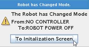
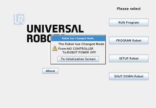
It is also possible to use the mouse and click on the
OK or “To Initialization Screen”.
From this stage on and the rest of the manual
a mouse click is used instead of pressing the touch screen monitor if not
mentioned otherwise. (The mouse click or press with finger has the same
result).
This will take you to the “Initialization”
screen because at this point just after a cold reboot the robot does not know
where the joints are situated. This also apply if the robot has been used and
programmed before – after a cold reboot this initialization is necessary for
the robot to find the position of the joints.
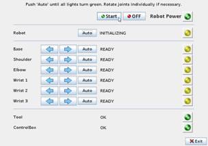
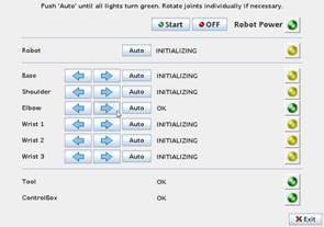
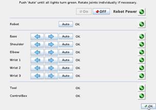
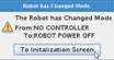
Notice that the screen say “Power OFF” and all
six lamps for the joints are yellow. The controller has power ON of cause, but
the robot is still Power OFF.
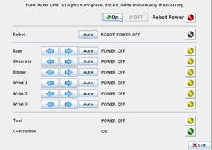
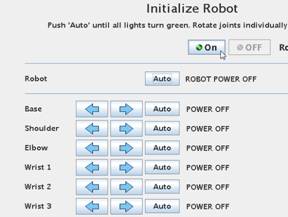
Press the “ON” button to turn on the power to
the robot.
The status will go to “READY” for each joint, but the
lamps are still yellow because the position of the joints is still unknown to
the robot controller.

Press the “Start”
button. You will hear six clicks – click – click – click – click – click which
are the mechanical breaks inside the joints that are releasing. The mechanical breaks
are use in transportation and after an Emergency stop to ensure the robot
joints do not move.
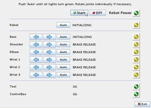
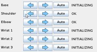
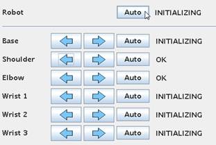
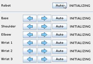
After a short
time you will see the “BREAKE RELEASE” go to “INITALIZING” status for all
joints. In some firmware version you will also shortly see the messages
“BOOTING” for the joints
The robot does
still not know the position of the joints and we have to help the robot on the
way in order not to crash into something (including into itself) when the robot
starts moving.
Because we have just unpacked and the robot is
folded together in a tight position we will use a very controlled method this
first time. Later we will see how a shortcut can be made when the robot is cold
started for a position where the robot is fairly free and unfolded.
In this position
we need to make sure the robot is moving “upwards” so it is not crashing into
itself. If it crashes into itself it will stop with a safety stop, but the robot
could be slightly scratched and we want to avoid that especially when it is
new.
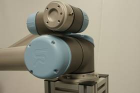
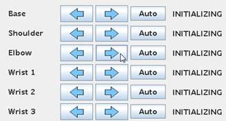
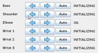
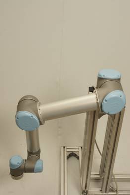
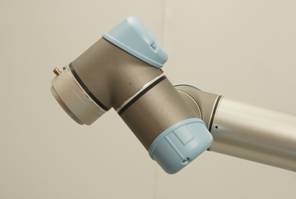
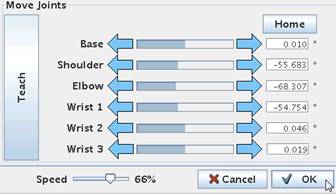
The robot is a 6 axis robot which means it has
six joints and six axis freedom of movement. The joints are named 0, 1, 2, 3, 4
and five counting from the base – or with names it is Base – Shoulder – Elbow –
Wrist 1 – Wrist 2 – Wrist 3.
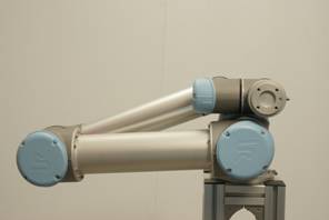
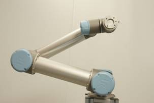
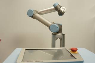
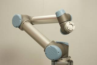
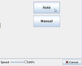
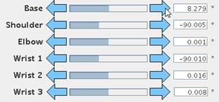
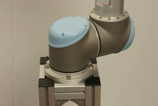
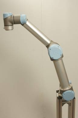
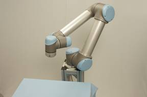
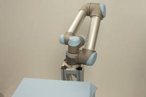
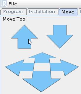
So in this case we want the elbow joint to
move upwards to make the robot freer. So press and keep pressing the arrow
pointing right – look at the photo at the right where to mouse pointer is
placed.
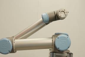
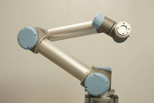
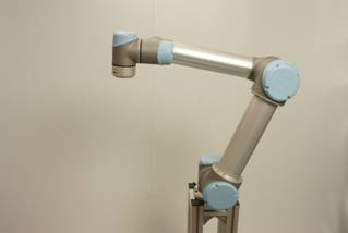
Keep pressing and
you will see the robot rise upwards.
After a few
seconds the “Elbow” joint will report “OK” on the monitor. This means the robot
now knows where this joint is positioned. It is not necessary to turn one full
circle. What you see on the photo is normal.
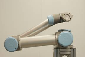
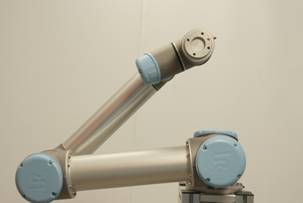
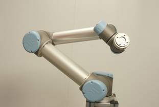
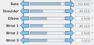
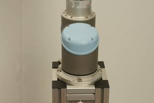
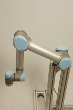
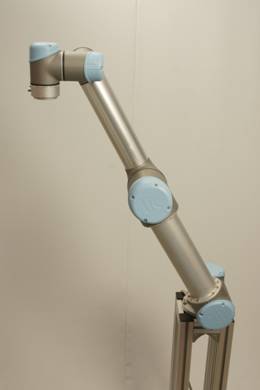
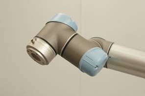
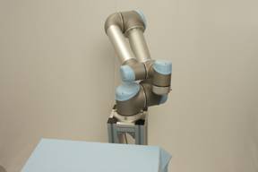
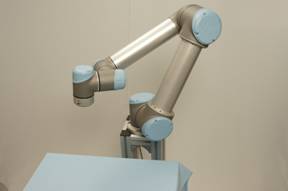
Now we want the
“Shoulder” joint to move upwards in order to get the more upright and if
turning down we might crash into the table if the robot sits on a table.
Press the arrow pointing to the left for the “Shoulder”
joint.
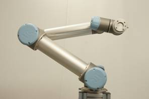
You will see the
robot move further upwards by the “Shoulder” joint movements.
After a few
seconds the “Shoulder” joint will also report “OK” and the position of the
joint is now know to the robot controller.
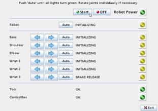
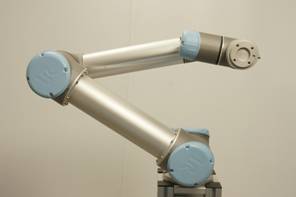
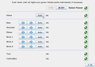
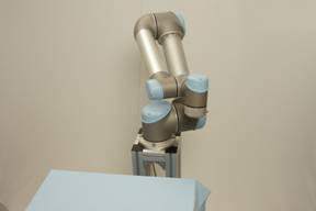
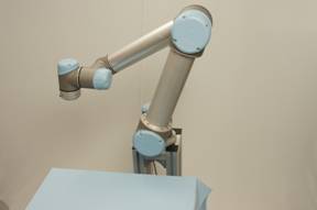
Now the robot is already quite good up and
free so for the last 4 joints we will use a faster method. Press the “Auto”
button on top of all joints where it says “Robot”.
Keep pressing the
“Auto” button. Now notice how the remaining 4 joints all move until all of them
say “OK” which means the robot has been Initialized and all joint position are
know to the controller.
This “Auto” method is actually possible for
all 6, but since the robot was folded we choose this controlled method until
the robot had more space. We will try that very soon the second time we start
up the robot.
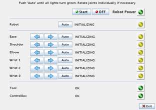
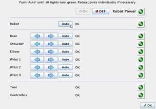
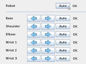
All the joints on the monitor reports “OK” and
notice how all the lamps turned green. The robot is now initialized and ready
to be programmed or load a program if we already have made a program before.
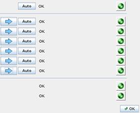
Press the “OK”
button at the bottom of the screen which takes you to a Main Menu screen.

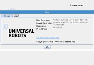
Try and press the “About” button. A screen
with software version information appears and if an IP address has been
assigned it is also shown in this screen. We will learn later how to set an IP
address so this is properly blank on your screen.

Press “OK” and you will return to the “Main”
menu.
For training purpose the shortcut method for initializing
the robot will be explained now because the robot is already up and free. So
shut down the robot by pressing the “SHUT DOWN Robot” button.
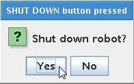
Confirm the
Shutdown by pressing “Yes” button.
After a few seconds the robot and controller
are turned off.
Notice how the six clicks could be heard
because the mechanical breaks engaged to make sure the robot does not fall
uncontrolled down to the floor.


Turn on the robot again following the same
procedure as explained above until you reach the “INITALIZING” screen.

Since the robot
is up and free then press the “Auto” button on the top where it says “Robot”.
Press only
briefly (0.5 – 1 second) and notice which direction the robot moves. Press
again only briefly (0.5 – 1 second) and notice again which direction the robot
moves. This is useful if the robot was power off near some obstacle or inside a
machine – then we can control the movement direction during initializing
because alternate press will cause the robot to go in opposite direction.
When you know the
direction of movement you wish the robot to go during the initializing
procedure then keep pressing until all joints report “OK”.
This time the initializing procedure went much
faster and this will often be the choice of method during a cold reboot of the
robot.
Press the “OK”
button at the bottom of the screen to go to Main menu.


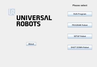
From the Main
menu next action can be selected. If a program is already available such
program can be loaded and Run directly from the “RUN Program” menu.
Or if we want to
program a new program we can choose the “PROGRAM Robot” menu.
Or we can go to
setup by pressing the “SETUP Robot”
Or we can
shutdown the robot which we already tried above.
In this case we
want to make learn more about how to operate to robot and therefore will go
towards programming the robot - choose “PROGRAM Robot”
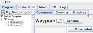
This will take
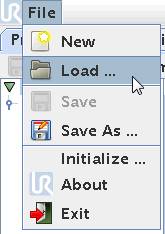
you to a screen where there is a “File” menu and 5 sub menu Tabs.
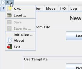
On is a “File”
menu from we have similar menus as the big buttons on the screen and from where
we also can load and run programs. This “File” menu will automatically be
explained as we progress this manual because we will be using this menu
frequently.
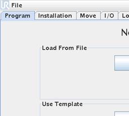
The 5 sub menus
below the “File” menu are called Program – Installation – Move – I/O and Log.
Try and press each of them just for now to briefly see what is inside each of
them.
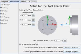
The “Installation
Tab is an advanced setup which will be explained later and is not necessary to
worry about yet.
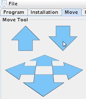
In the next chapter we will focus on the Move
Tab.
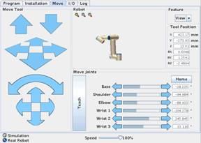
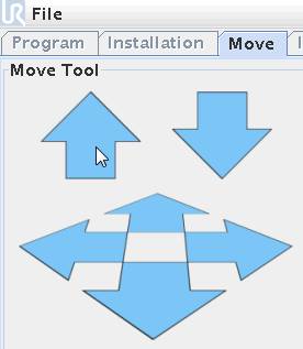
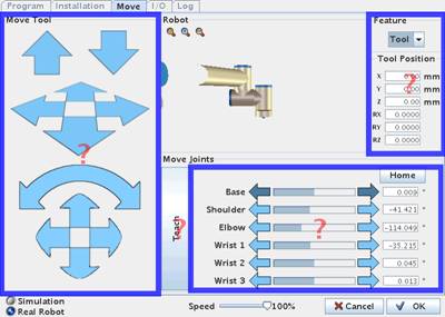
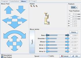
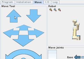
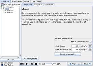
Press the Move Tab and you will see this
“Move” screen.
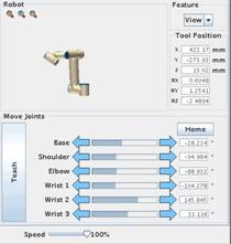
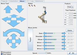
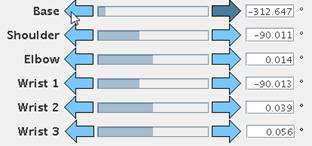
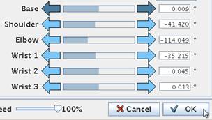
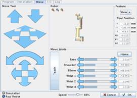
The screen has
several functions, but the main purpose is to move the robot around in its
space during programming and to get a report where the joints are located which
are shown on the degree position of each joint or above by the X – Y and Z
position indicator.
The arrow keys are the most frequent used. The
right side has six arrow bars which represent each joint and its position. Each
individual joint can be moved by pressing these arrow bars.
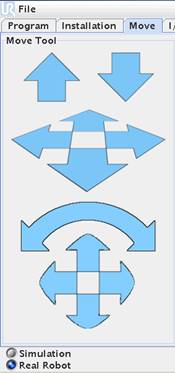
On the left side is “Combination” move
control arrows. These arrows move several joints simultaneously in order to
make linear moves during the programming phase. Especially the Up and Down
arrows are useful for linear Up and Down movements.
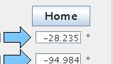
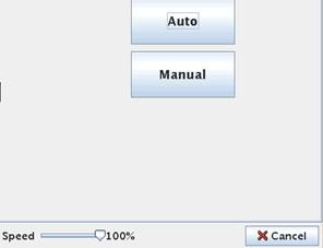
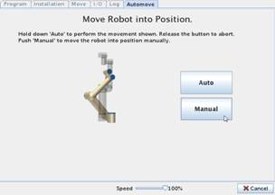
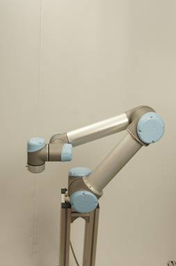
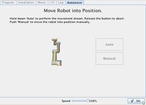
The robots
natural “Home” position is straight up in the air and the Move Screen has a
“Home” button. Press the “Home” button to try and position the robot into the
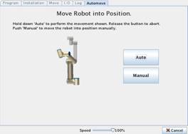
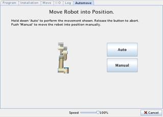
Home position. When pressing the “Home” button the robot will not start move
right away – instead we will see a “Move Robot into Position” screen because we
need to do it in a controlled way in order not to crash into something. We have
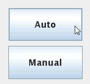
two options – either an Auto move or a manual move. When pressing the “Auto”
button the robot will start moving into its home position by it self as long we
keep pressing. Releasing the button will stop the robot move.
Notice that the button
in the lower right corner has a red X and reads “Cancel” and we can press here
if we want to return to the Move screen.
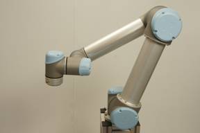
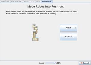
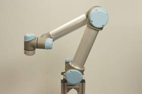
When the robot is
fully stretched i.e. in its Home position we will see the button in the lower right
corner go to “OK” with a tick symbol – which means the robot has reached the
“Home” position.
This is the Robots naturally home position,
but during programming you can choose any position to be your home position.
When running your program the robot will first need to go to your defined home
position which might be near where you want to have an action and not necessarily
this robot “Home” position.
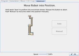
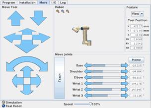
This is how the screen and robot looks like
when the robot reaches the “Home” position.
If there are
obstacles near the robot and there is a risk the robot will crash into these
obstacles during an “Auto” move – then you can choose a “Manual” move. Press
the Manual button instead - which brings you to the Move Screen. Here you have
full control of the robot movements by pressing the arrow bars and you can
safely guide the robot into the “Home” poison and away from obstacles.
Now the robot is fully stretched is a nice
position to start moving each joint to see how the robot moves. Start with the
base joint and press the Arrow bar left or right and see how only the base
joint moves.
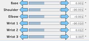
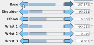
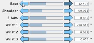
You can monitor the position of the joints by
observing the digits degree indication next to the arrow bar.
After turning the base joint around – this is
a good opportunity to fit our last bolts in the base if you have not already
done so.
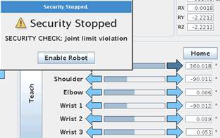
If you turn the
joints all the way and beyond its limitation you we will se an Error messages
“Joint Limit Violation” which is a safety stop in order not to spoil the inside
of the joint. Press “Enable Robot” to acknowledge the error messages.
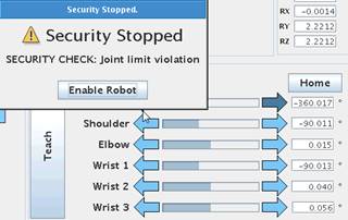
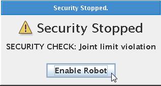
The same error messages occur when you turn
the robot joint 720 degrees all the way to the other side. Press “Enable Robot”
to acknowledge the error messages.
Notice how this part of the arrow bars handles
each joint individually.
The left side of the Move Screen also has
arrow keys to control the robot, but this side will perform a movement in
relation to the tool head position. For example straight up or down
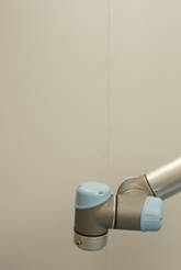
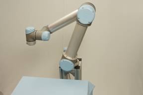
The robot moving
towards the floor.
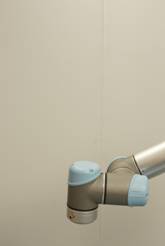
Press the “Up”
arrow and get the robot back up again. Continue to press up all the way up and
observe the robot.
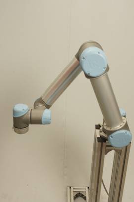
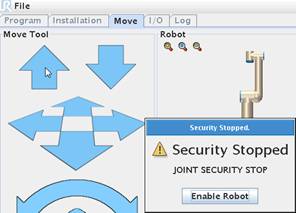
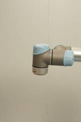
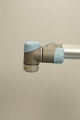
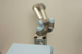
Almost fully stretched. Fully
stretched and security stop.
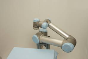
You might notice that when the robot was very
near to the top and at its limitation the speed seemed to accelerate just
before the robot stopped with this “Joint Security Stop”. The security stop is
obvious because the robot was following a straight line upwards and now the arm
is fully stretched and it is not possible to go further up because of the
physical length of the arm and therefore the security stop.
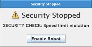
The phenomena regarding the slight speed
acceleration just before the Security Stop is called a Singularity because the
mathematically calculation and physical movement of the joint is reaching an
illegal mathematical expression which is called a Singularity.
You can experience this also in your
programming especially in MoveL (linear move mode) when you have set two
Waypoints that are impossible to connect in a linear line because it would
require a mathematically and mechanical illegal move and therefore you might
experience such phenomena in programming called a Singularity – and the robot
stop with this error messages. More about this later during explanation of
MoveL programming.
 Singularity security stops.
On the left side
on the Move Screen below the Up and Down arrow keys are a set of arrow keys
that can move the robot in relation to the tool head position.
The tool head position is our references in
most cases and our X, y and Z position because we often need to do our action exactly
and the tool head position where our tool is mounted.
With these arrow keys the robot can be
manipulated in relation to this tool head position which can be useful if you
want to keep the position of your tool, but wish to move the robot arm to
another posture, but with same target object as reference.
The speed adjustment”
accelerator” 0 – 100% is meant for commissioning and troubleshooting. It is
very useful to use when the robot is being manhandled and to check “what is
really going on” in slow motion. But a funny thing to be aware of is that if
you have made “Wait” instruction in your program – let’s say Wait 3 seconds –
and then if you turn your speed down to 50% - then guess what – your wait
instruction became 6 seconds – maybe not what you expected.
During normal run
– you need to program your intended speeds and run it at 100% – it is better
programming method.
But the first time you test run your program
and robot near your other machine or packing line – then it is advisable to run
at a slower speed in order to have more time to react and stop the robot if the
program and move did not follow your intention.
![]()
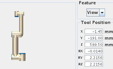
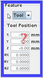
On the right hand of the Move Screen is the X,
Y and Z numeric position of the robot and tool head. This can be useful
especially in Script programming mode.
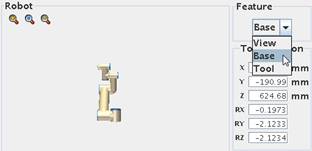
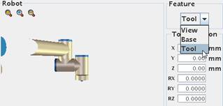
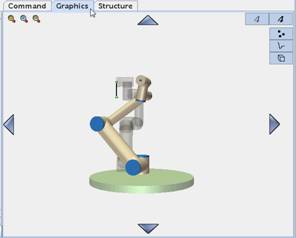
In the middle of the move screen is a graphic
representation of the robot position which is useful as a guide for the robot posture.
You can choose between two different views (Base view or Tool view) i.e. angles
of the graphic representation.
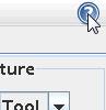
If a screen has a “?” in the top right hand
corner means that a help screen is available. Press the “?” and the screen will
be divided into boxes.
Point and press on the boxes you where you
wish to read some help information’s.
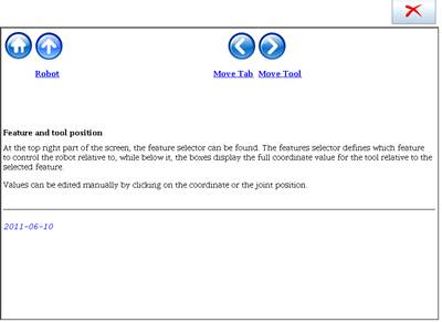

After reading the Help information – press the
red “X” to return to the previous screen.
The Universal-Robot is ideal to use in a small
cell for automation because the control besides the robot programming environment
also comprises of inputs and outputs which also is easy to program from the
onscreen programming environment.
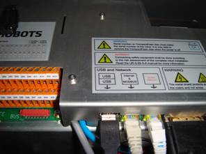
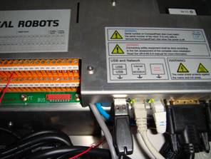
The robot has a standard 8 digital inputs and
8 digital outputs on the controller board inside the cabinet along with 2
analogue inputs and 2 analogue outputs inside the cabinet.
Additional there are also 2 digital inputs and
2 digital outputs and 2 analogue inputs on the tool head itself. This is very
elegant because the cabling for these interfaces is routed inside the robot and
therefore no external cabling is necessary for these interfaces.
This means that external equipment that is
connected to these I/O interfaces like conveyor belts or actuators can be
controlled and program from the robot.
If you need more input and outputs then is
also easy to extend the number of I/Os by using MODBUD nodes connected via IP
network. See later in the manual how to connect and configure a MODBUS node.
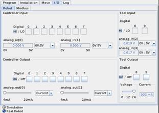
To monitor the status of the I/O signals the
I/O tab is very useful. Each I/O is represented by a box that is “off” is the
signal is “low” or the box is dark if the signal is high.
The out puts can also be manipulated i.e.
overruled during commissioning and testing phase in order to check the
connected external equipment.
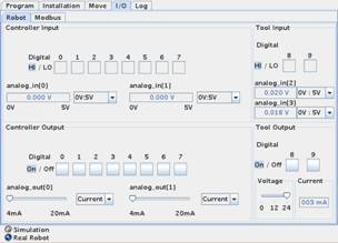
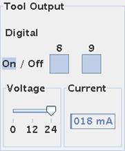
Overall status of I/O. Input 8
and 9 on the tool head is both “high” in this case.
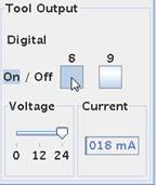
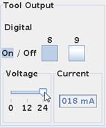
Toggle output on/off by pressing the
box at Output 8 is “On”.
And it is 24V. The “meter” shows
the output. The
device on output 8 is dragging 56 mA.
Digital Outputs are Open collector type. Open
collector means that the outputs are implemented to ”sink” and we can say they
are ”Active low” because connecting an actuator can be done by applying the
supply voltage at the ”far” end of the actuator connections and the other
connection to the output terminal - and then when the output is driven low by
the programmer – the external device turns on.
If you prefer to
have an ”Active high” output – it is also possible – then just apply a ”pull up
resistor”. So now the ”far” end of the external device is connected to GND and
the other end is connected to the output and a pull up resistor. The pull up
resistor is connected to the supply voltage. Now when the output is driven
”high” by the programmer the external device turns on.
Open collector is
actually an advantage because it gives the implementation more choices.
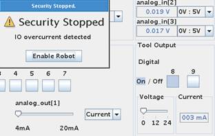
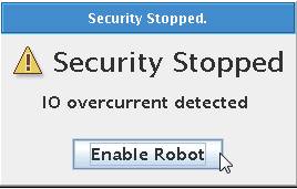
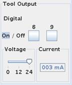
The output is not current limited, but if the
output is short circuited it will result in a security stop and error messages
because of over current detected on an output.
Press “Enable
Robot” to restart.
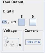
Notice that after
an Over current Security stops the voltage is reset to 0V. This has to manually
be set back at the desired output voltage 24 V in this case by pulling the bar
after the short circuit condition has been removed.
The voltage for
the I/O on the tool head can be adjusted to 0 or 12V or 24V from this I/O Tab
Screen.
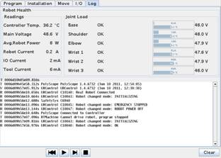
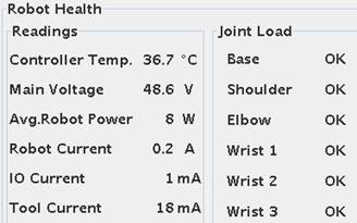
The log Screen can be reach by pressing the
“Log” tab. The log screen provides useful information’s about the status of the
robot and controller.
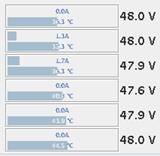
Information’s for controller temperature,
consumption, power supply output and joint status is available.
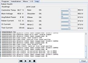
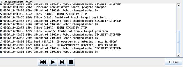
Below is a
running system log with information of resent status and activities. The
control buttons are available for running or single step the program and the
log entries can be observed while running which is useful for troubleshooting
purpose.
The robot can be programmed in different ways.
From this onscreen method or remotely by script programming. In this chapter we
use the user friendly touch screen method.
The robot has two ways of calculating how to
move from Waypoint to Waypoint which is a Non linear movement (MoveJ) and a
linear movement (MoveL). The “J” symbolizes the rounded nonlinear move mode and
the “L” symbolizes the linear move mode. The non linear (MoveJ) is the default
and the most commonly used and the one to recommend using if it is not
absolutely a must to use a linear move. The difference is the way the robot
calculates and how to move to next position. In the non linear (MoveJ) method the robot
might seem to take a slight bended route from point A to point B – this is
because of the physical construction of the robot – the lengths or “arms” and
“wrists” combined with when the motors are turning. This is normally not an
issue in normal pick and place operation and can easy be overcome by inserting
more waypoints – like mentioned above.
But if you want the have an absolutely perfect
linear move from point A to point B it is possible by using linear move
(MoveL). However the downside to this that turns and smooth bends now become
more difficult to perform. In pick and place you properly need to go in and out
up and down and around most of the time and a linear move is not important – so
MoveJ is recommend to use.
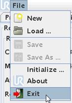
From wherever you
are in the menus – Press “File” and “Exit” to return to the Main menu.

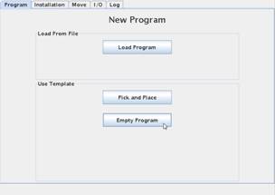
Choose Program
Robot
and select “Empty
Program”.
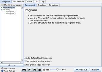
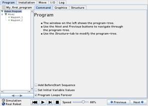
This screen is the program screen and properly
in the future the screen you will be at most of the time. This is where you
build up your program and test run it.
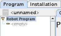
The left side is the program window where the
program statements are inserted line by line downwards.
At the moment the
program block is empty and empty. That’s why the test is yellow because nothing
is defined. We can also it says “unnamed” because we have not loaded or named any
program at this moment, but very soon we will make a small program.
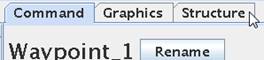
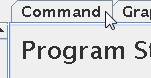
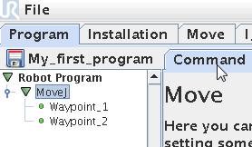
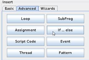
In the middle there are 3 tabs – Command – Graphics
– Structure. We are actually in the Command tab already and that’s why it is
highlighted.
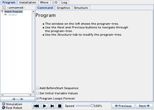
Below is 4 control buttons which looks like a
CD player which we will use when we start our program later. There is also a
“Speed” indicator from where the speed of the robot program can be manipulated.
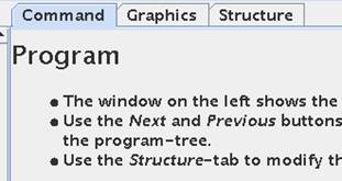
The “Command” tab
and the “Structure” tab is properly the most used tabs on the robot control and
programming the robot is a frequent use of “Command” and “Structure” tab.
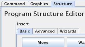
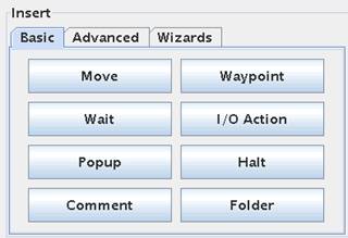
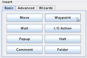
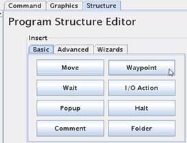
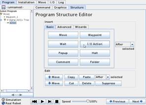
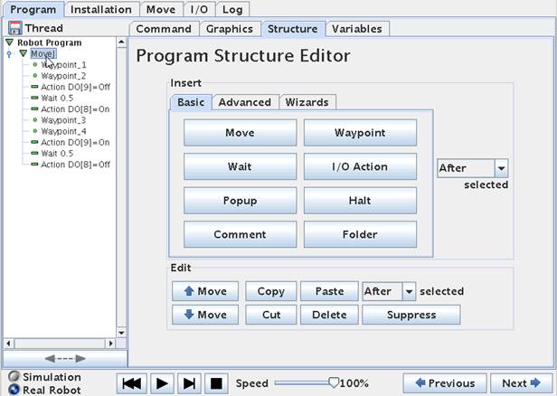
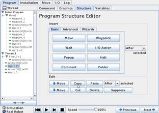
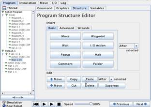
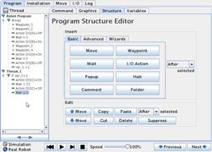
Press the
“Structure” tab. This brings you to the first of 3 different program objects to
choose from when we build up our program.
The very first thing we need to do I robot
programming is to define our path and movement for the robot. This is done by
defining Waypoints (positions). So we define the positions the robot has to go
through rather than the actual path. In other words we choose a position e.g.
“A” and next position e.g. “B” and then the robot will calculate how to come
from “A” to “B”. (Not to be confused with that the robot records the path we
moved the robot by hand or by control.
Let’s get started to program and now choose a
Waypoint. Pres the “Waypoint” button.
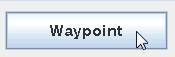
Ups we already
got an error messages that says “Waypoint has to be under a Move”.
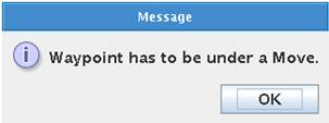
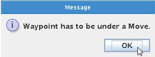
So we need to go
back to the program screen – Press OK to acknowledge the messages.
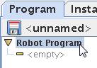
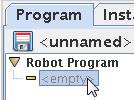
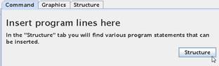
We need to be in
the section where we can insert program lines – so point and press on the
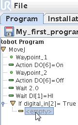
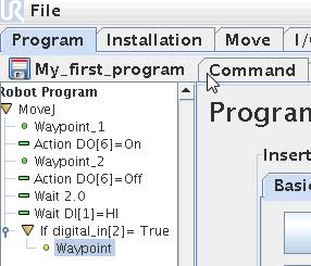
“empty” word so it becomes highlighted.
Now again Press
the “Waypoint button.
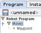
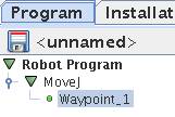
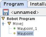
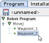
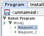
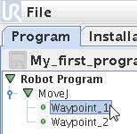
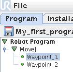
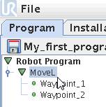
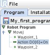
Notice how a
“MoveJ” and “Waypoint” has been inserted and it starts looking like a program
tree. The statements are still yellow because we have not defined the position
of this Waypoint.
MoveJ is the default and that’s why this is
automatically chosen for us here. Later MoveL will be explained.
This first Waypoint is also what becomes this
user program “Home” position and this can be anywhere and therefore different
as to the robot home position discussed in the Move Screen.
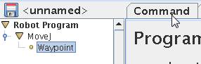
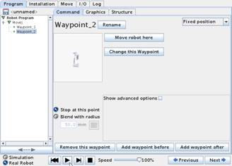
We need to define
each Waypoint we insert into out program. Point and press on the Waypoint we
want to define – in this case there is only one because we just started
programming. Press the “Command” tab.
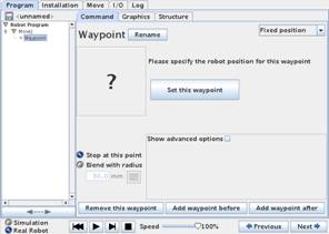
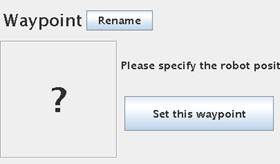
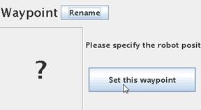
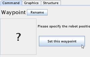
Because we have
pointed out the Waypoint in the program tree we now get this screen with a big
“?” question mark – like it is asking us where should this waypoint be ?.
So we need to set. Press the “Set this
Waypoint” button.
This brings us
the familiar Move Screen.
We can choose to use the Move Screen
to move the robot
into position by pressing
the arrow keys on
the bars.
But the arrow keys are more useful when we
need to fine adjust our Waypoints. Here in the beginning to define our rough
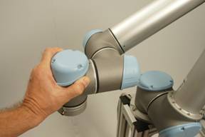
positions it is faster to use the “Teach in mode” by moving the robot by hand.
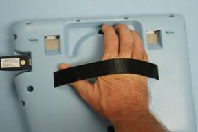
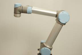
On the back side of the monitor there is a
small button. Hold the monitor as shown on the photo with one hand because then
it is easy the watch and handle the monitor and also to press the button on the
back of the monitor.
This small black button releases the breaks on
the robot and you can now move the robot into position by moving with your
other hand – a little effort has to be made to move it because we also don’t
want to drop on the floor. (This can still happen if a heavy tool is mounted on
the robot head).
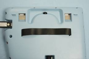
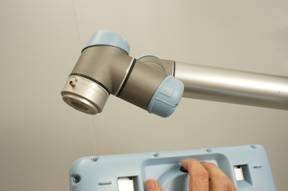

Press and keep pressing the black button on
the back of the monitor and grab the robot and start moving into your desired
position.
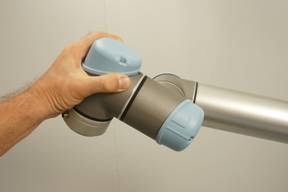
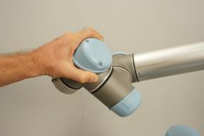
When you are happy with the position then
release the black button on the monitor again
While we were manually manipulating the robot
around with our hand we had the Move Screen on the monitor. Press the “OK”
button in the lower right corner of the Move Screen which takes you back to the
Program window.
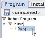
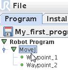
Notice how the
Waypoint and the other symbols turned green because now we have defined the
statement which is the Waypoint. Actually we already have a very small program
because all symbols are on green, but a program with only one Waypoint is not
funny to look at because it will not move the robot.
So let’s define one more Waypoint.
![]()
Press “Structure”
to go to our program object menu. Choose “Waypoint” again.
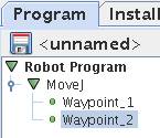
The second Waypoint has entered into the
program, but it is still yellow because it is undefined, make sure you have
highlighted the yellow Waypoint statement. Press “Command” to define the
Waypoint.
Press “Set this
waypoint” which brings up the Move Screen. This time we just choose to move the
tool head upwards with the “Up” arrow key.
Keep pressing the “Up” key until the robot
reaches a desired
position and the release
the “Up” key in the Move Screen.
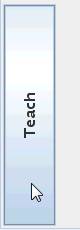
The “Teach” block in the Move Screen has the
same function as the black button on back of the monitor i.e. to release the
robot breaks for manual manipulation into position.
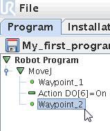
Press “OK” on the
Move Screen to go back to the Program tree window. Now we have two green Waypoint
in our program.
The controller software checks the syntax for
us automatically and that’s why we have green symbols which mean our syntax and
method is OK.
![]()
We are ready to test run our first program.
Press the “Start” button (The triangle symbol). The program does not start
executing right away because we left the robot in the Waypoint 2 position
whereas Waypoint 1 is our “Home” position. Before we can start the running the
program we need to bring the robot to this “Home” position – and therefore a
Screen appear when we can move the robot either automatically or manually.
Automatically is the easiest if the robot is
free fro obstacles, but if we need to guide the robot we can also choose the
manual method.
Notice how the
button in the lower right corner has a red “X” and says “Cancel” because the
robot is not yet in the “Home” position. The graphic also shows how the robot
has to move from its current position to the “Home” position.
Make sure the
robot is free from nearby obstacles.
Press and keep
pressing the “Auto” button and observe the robot movements towards the “Home”
position.
.
This programs “Home” Position.
When the robot
reaches the “Home” position the button in the lower right corner of the Screen
goes from “Cancel” to “OK”. When it says “OK” the Press ok.
![]()
Press Start (The black triangle
symbol).
Program tree Screen.
After pressing
the “OK” button the program tree Screen reappear, but the robot is still not
moving, but now it is in the “Home” position and can be started.

The robot runs
the program by it self from Waypoint_1 to Waypoint_2 continuously. This is just
an Up and Down movement.
![]()
![]()
You can stop the
program execution. You
can pause the program execution.
![]()
![]()
You can restart
the program execution. You
can control the speed during test run.
Notice how you
can follow the program execution during the program run so you now where in the
program the robot is.
The Speed regulator is useful for testing.
During normal Run it is better control you speed in you program because the
Speed regulator will slow down everything in the program inclusive of wait
statements.
The teach pendant
looks like a Tape recorder or CD controls i.e. Play – Stop – Pause - and Step
buttons.
The Single step
button is also for commissioning and trouble shooting because when you single
step through your program it is a Single step of Program lines. So again – if
you expect your program to be executed when single stepping – you will be
surprised because the conditional expressions will maybe not be executed as
expected – e.g. if you have programmed that a subroutine should only be
performed when an input is High. But then when you single step your program –
the robot will follow your commands step by step move from waypoint to waypoint
when you single step.
![]()
![]()
The speed adjustment”
accelerator” 0 – 100% is meant for commissioning and troubleshooting. It is
very useful to use when the robot is being manhandled and to check “what is
really going on”. But a funny thing to be aware of is that if you have made
“Wait” instruction in your program – let’s say Wait 3 seconds – and then if you
turn your speed down to 50% - then guess what – your wait instruction became 6
seconds – maybe not what you expected.
During normal run
– you need to program your intended speeds and run it at 100% – it is better
programming method.
![]()
The “Wind” back control
can be used to move the cursor while programming back to the top of the
program.
After writing a few lines of the program it is
advisable the save your work. As explained early in the manual it is good to
assign a USB drive for this purpose.
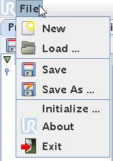
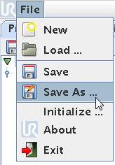
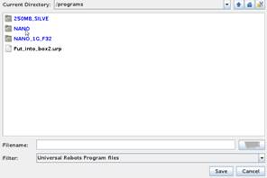
Press the “File” menu and choose “Save As …”.
![]()
A Screen with
file structure and files already present on the Hard drive (Flashcard) appears
and the USB drive is already shown as a Directory. The controller recognizes
the USB drive automatically.
In this case the
USB drive has the name “”NANO_1G_F32” which was a name I give it while it was
sitting on my office computer, but this can be any legal computer file name.
Sometimes a USB drive has a default name when it is purchased and sometimes it
is just without a name so you might see other names or even “unknown”. This is
not important as long you know it is the USB drive you inserted to the robot
controller.
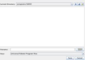
Press on the name “NANO_1G_F32” to go into
that directory i.e. go to the drive.
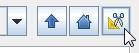
If the USB drive
is empty there are no directories on the USB drive and you can use the scissor
symbol to create a directory. If there is already directories from where it was
in your office computer then will be shown on the Screen and you can chose to
go to the sub directory. Here we will create a sub directory.
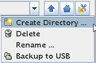
Press “Create
Directory …”
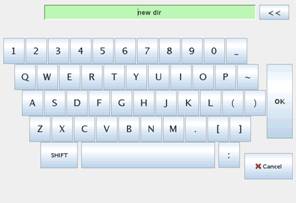
The controller
suggests “new dir” as a name, but better to choose something else that says
something about the content of the directory.
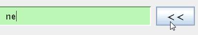
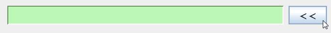
Press behind the new dir name and use the
<< button to delete the “new dir” name.


Use the onscreen
keyboard to create a new name e.g. Test
in this case.

![]()
![]()
Press “OK” when
finish the name.
A new directory
called “Test” appears. Press on the “Test” directory to go into it.
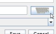

Press the on
Screen keyboard symbol to type in your desired file name for your program. In
this case we call it My_first_program.
If you have connected a keyboard along with
the mouse, then you can use the keyboard to key in which is much more
convenient.
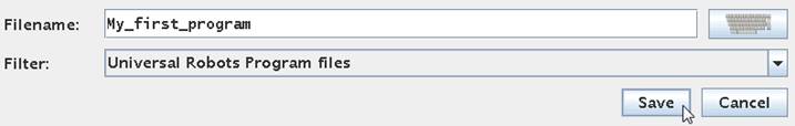
Press “OK” when
finis typing. Notice after pressing “OK” the file name is listed below on the
Screen.
![]()
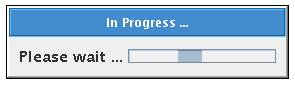
Press “Save” to
save the file and a popup messages appear to confirm the save of file.
After the
controller finish the save it returns to the Program tree we were working on
and we can continue programming which will be explained in the next chapters.
![]()
To load back a
program that we previously have saved on the USB drive press the “File” menu –
choose “Load”. Press on the name for the USB drive (in my case NANO_1G_F32). If
you choose to create sub directories then go all the way down to your file by
pressing the sub directories until you see your file you wish to load.
![]()

![]()
![]()
Press on the file
so it is highlighted. Press on the “Open” button.
You will see your
program reload into the Program tree block and you can continue to edit the program
or simply use the program if is a finish ready made program.
Between the “Command” tab and the “Structure
tab which we have used a lot so far is the “Graphics” tab. Press the “Graphics”
tab.
This window shows a Graphic representation on
the robot during program run like a 3D simulation.
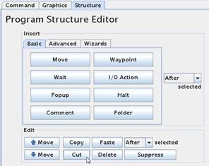
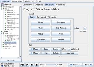
In the “Structure” Screen at the bottom is
normal Cut and Paste functions which is very useful when program parts has to
be moved during program edit or completely Cut away.
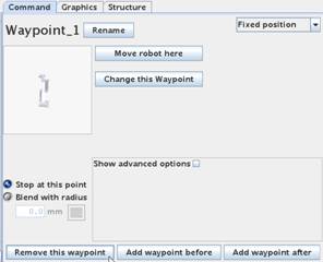
The “Command” tab
also has a few edit functions for adding or removing Waypoints.
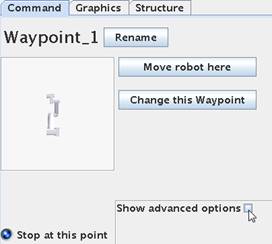
When highlighting
Waypoints in the Program block then the “Command” tab also have a function
called “Show advanced options” try and tick that option.
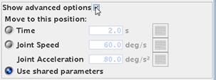
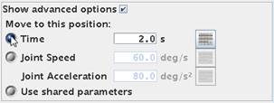
This is used to define how fast the robot
should move. Each Waypoint can be defined for how fast the robot should reach
there from previous Waypoint.
This setting can be defined as pure time as a
formula of the joint speed and acceleration.
Be aware of that if the speed is set low in
relation to how far the two Waypoints are from each other then the robot might
try to speed up and run too fast which will cause a Security stop to be
activated.
To learn about
the MoveL linear movements we will just continue using the program we created
in the last chapter called “My_first_program.urp”. Maybe you need to Load the
program into the controller as described above – or simply make a new small
MoveJ program as explained in previous chapter.
Because we will just change the MoveJ program
into a MoveL program.
So you will have this small program on the
Screen
Point on the
MoveJ statement and Press so it is highlighted.
If not already in
the Command view then - Press the “Command” tab.
Then you will see
the definition screen for the MoveJ statement. We can also call it the
properties for the MoveJ statement.
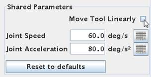
At the right hand
side lower corner is the definition for the MoveJ statement which by default is
a nonlinear movement hence the MoveJ statement in our program.
Below is a
parameter called “Move Tool Linearly” with a check box – Check it.
.
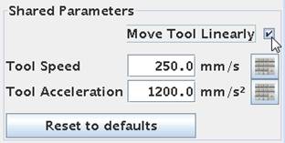
Go back to the
Program tree Screen and notice how the MoveJ statement has changed to a MoveL statement.
Remember that the
Waypoint_1 and Waypoint_2 is the exact same as in the previous chapter.
Now we can
compare the different movement for these two programs.
The programming environment and object to
choose in MoveJ and MoveL are the same which is already explained in the
previous chapter – so how to start and run the program is the same.
Run these two
programs after each other to compare – now press start for this MoveL program –
move the robot to the “Home” position and Press start again and see the
movement.
Reload the MoveJ
program and Run that program.
See the
difference ?
See next page.
MoveL MoveJ


MoveL MoveJ
Notice the
difference for a MoveL to a MoveJ movement. The middle picture for the MoveJ
shows the tool head out fro the centre line. Whereas the tool head stays at the
centreline during the MoveL move.
In pick and place the MoveJ is advisable –
only rarely a MoveL is necessary.
As I described previously when using the MoveL
programming method there is a change to run into a Singularity which is an
illegal mathematical expression.
To illustrate that I have made a quite stupid program.
I am using the exact program as above i.e. only two Waypoints in the MoveL
mode. The two waypoints I have chosen are seen below.
Waypoint_1 Waypoint_2
Since I have chosen MoveL I expect that the
robot goes in a straight line from Waypoint_1 to Waypoint_2, but notice that it
would require the robot to go through the base joint at the centre because the
two points are on each side of the base.
But I have been able to make the program and
all statements are on green so let’s try to run it.
The robot started
to move from Waypoint_1 towards Waypoint_2 in a straight line, but when the
physics was in the way the robot showed the phenomena about increasing in speed
and then rapid security stopped with “Speed limit violation” and never reaches
Waypoint_2.
Let’s just try
and change the above program to a MoveJ program with the same Waypoint_1 and
Waypoint_2 positions and run it.
The robot runs this program beautifully
without any error messages in MoveJ mode because it is allowed to take a
bended route from Waypoint_1 and Waypoint_2
When using the robot the movements is
important, but evenly important is to be able to handle inputs and outputs so
the robot can react to external conditions and grab and hold items and feed
back when the robot finish its task. Therefore the controller software also can
handle such I/O interface and this chapter will explain how to set an output and
how to read an input and take an action based on such inputs status.
We will continue to use our program we already
started on – or you might wish to start a brand new user program.
This example starts with a program that
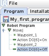
already has two simple Waypoint position like our “My_first_program.urp”.
Since we already have to program lines then we
need to decide where we want to have out action. In this case we want it in
between the two Waypoints so we place the cursor by pressing the first
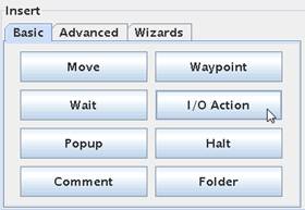
Waypoint. Press the “Structure” tab. This time choose an “I/O Action”.
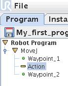
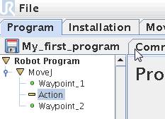
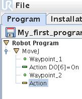
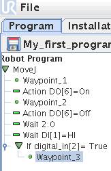
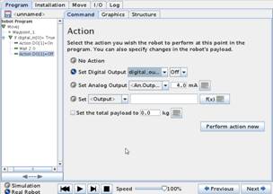
This causes an
“Action” statement to enter our program. Still yellow because it is not
defined. Make sure the “Action” line is highlighted and Press the “Command”
tab.
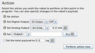
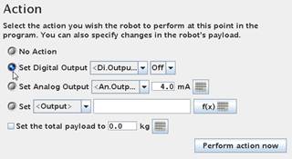
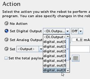
We need to define
the action. In this case we want to set an output – so tick the “Set Digital
Output” bullet.
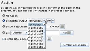
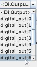
We need to choose
the output number to set. In this case we choose digital_output[6]
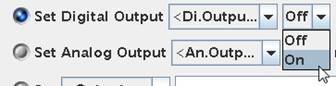
Along with the output number we have to define
the status we want to output to be set to. (High or Low) (On or OFF). Try and
choose ”On” which will set the output high.
Notice that the “Action” statement line turn
green and the output name and action associated with it which means it is now
defined.
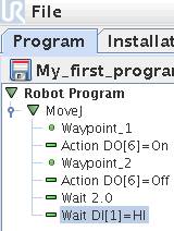
Continue
programming we wish to control the same output after the robot has moved to the
Waypoint_2. Press the Waypoint_2 and go to “Structure” tab and pick one more
I/O action.
Press the
“Command” tab and again choose “Set Digital Output” and select
digital_output[6], but this time set it to OFF.
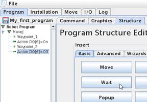
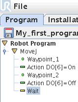
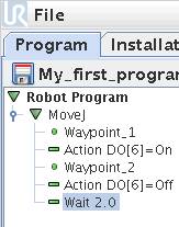
Continuing programming we wish to have a Wait
instruction at this stage in the program. Press the “Structure” tab and choose
the “Wait object.
Now a “Wait” statement enters the program
block. Make sure the Wait is highlighted and Press “Command” tab to define the
“Wait” statement.
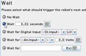
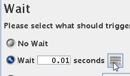
In this case we
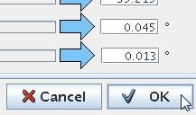
want to have a flat Wait based on time for 2 seconds. Tick the “Wait 0.01
seconds” tab. Press the “Keyboard” symbol in order to define the Wait time.
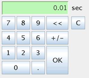
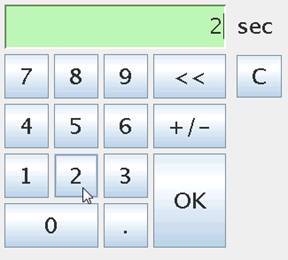
The Wait time is
pr. Default set to 0.01 sec, but you can set it to a new value e.g. 2 seconds.
Press “2” and “OK”.
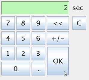
Now the “Wait” statement turned green and is
defined as 2 seconds.
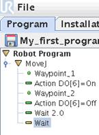
A wait can also be defined as a Wait for a
condition to happen e.g. a change in an input status. Press “Structure” tab and
insert one more wait instruction.
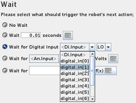
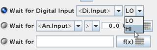
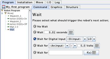
Press the
“Command” tab in order to define the “Wait”, but this time choose “Wait for
Digital input”. Select digital_input[1] and select the status “Hi”. This means
the program will wait until this condition occurs. This could be a signal from
an external machine we are interacting with.
In our program
block the second “Wait” statement also turned green because it is defined –
although this Wait behaviour is different as the first one.
This “Wait” instruction we just made because
the program to stop until this condition occur. Sometimes we still want to do
other things while we are waiting for these conditions to occur. In such case
we can choose an “IF” statement instead.
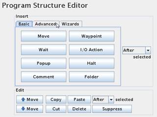
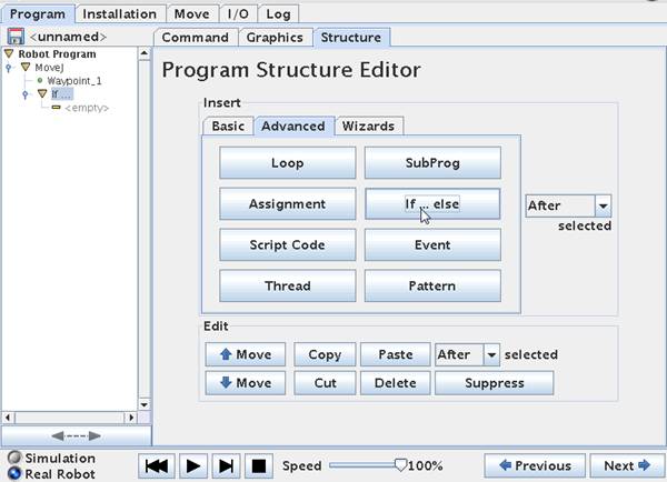
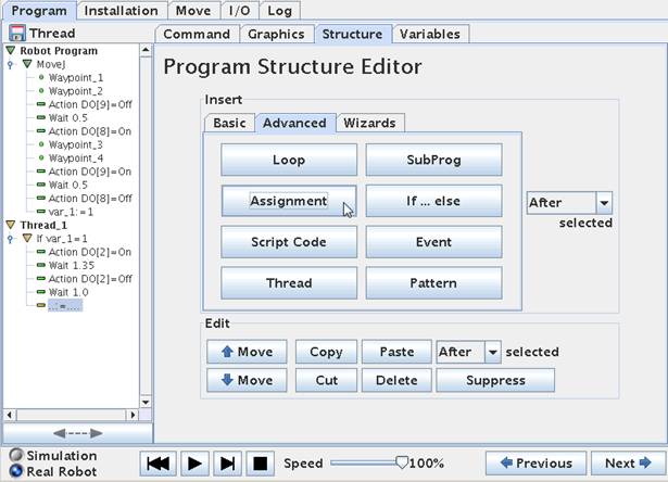
Press the “Structure”
tab. Inside the “Structure” tab is three sub tabs. So far we have only used the
Basic one. This time Press the “Advanced” tab.
Inside the “Advanced” tab is more program
objects to choose from. Choose the one that say “If … Else”.
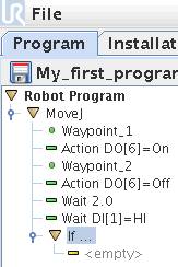
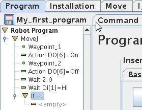
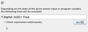
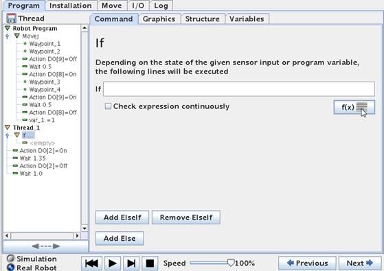
Notice how the “If ..” statement enters our
program block. Still yellow because we need to define it. The “If” statement
actually has two yellow markings because we need to set to parameters for the
“If”. First the condition for the If to happen – and what to do when the “If”
happens.
Make sure the “If . .” line is highlighted. And Press the
“Command” tab.
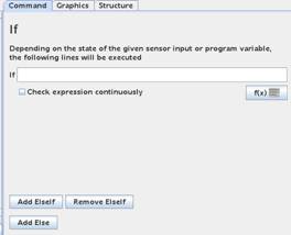
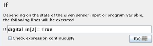
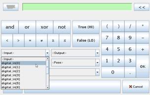
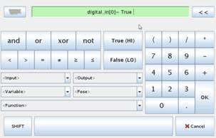
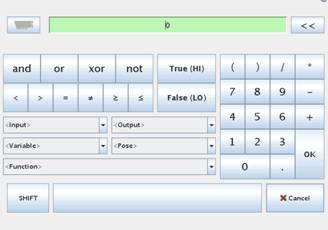
Now a Screen appears that has a “Formula” line
because we need to set the formula for the “If” to react on. Press the f(x) formula
tab.
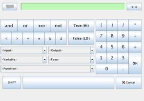
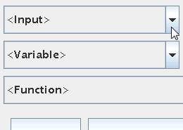
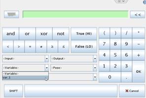
Inside the
“Formula” screen is several functions to choose from. In this case we are
looking at an input we want to react to. Choose the “Input” function.
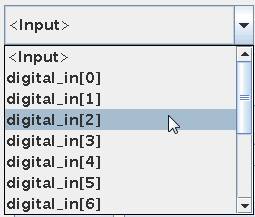

We need to choose the input we are looking at.
In this example Choose digital_in[2]. Notice how the input name appears on the
formula line at the top of the Screen.
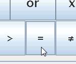
We need to finalize
our formula and make it a condition – for example choose the equal sign.
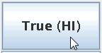

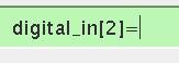
We want to react when this digital input 2 is
“high” so choose “True (Hi). (The level of a digital signal can be expressed as
0, Low or False for a 0V signal or High or True for an active signal. The level
of the high can change depending of if we are using 12V or 24 control voltage.
Press “OK”. The
formula line has now the condition for the “If”.
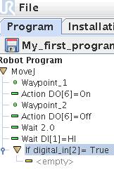
Also in the
Program block the If statement became complete, but it is still yellow because
the Action part of the If statement is empty i.e. not defined.
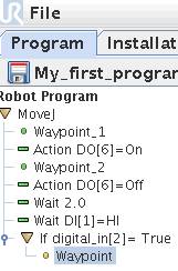
Make sure the second part of the If statement
is highlighted – in this case the “empty” line.
Press the “Structure” tab is order to choose
an object for our action when the If expression becomes True. For example
choose a Waypoint so if the If statement becomes true the robot will go to this
Waypoint.
In the Program
block the second part of the If statement now have a Waypoint as action. And
the Waypoint needs to be defined just like all other Waypoints. Make sure the
Waypoint line is highlighted and Press the “command” tab.
Now define the
Waypoint just as normal described in the previous chapter – either by hand
teach mode or by using the arrow keys.
When satisfied with the Waypoint position – then Press “OK”.
In the program block the Waypoint now becomes
green and all statements are defined and the program is ready to run.
In programming one of the most used features
is the IF or conditions based statement because that’s the hearth of automatic
choice of conditions and this is very often then main purpose of computer
program.
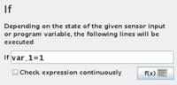
In the UR we have the IF statement to use.
Insert an IF statement into the program
Define the IF
statement by clicking on the formula button.
This will bring up a screen where we can
choose conditions for the IF statement to check on. In this case we choose an
Input to check on.
In this case it means that if Input 0 is true
the IF statement is true and the lines in the IF statement will be executed.
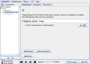
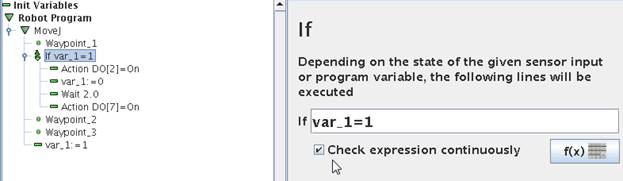
Below the IF
expression definition field is a check box called ”Check expression
continuously”
If this is checked the robot will check IF ”digital_in[0]”=
True is true also during the execution of the program lines in the IF statement.
This means that if the ” digital_in[0]” becomes 0 during the IF execution then
the rest of the program lines inside the IF will not be executed. This can lead
to unintended function if not handled correct.
Below the IF statement program lines is to be
inserted that will be executed if the IF statement is True. This can also be
considered a program inside the IF statement and it can be as big as our main
program, but often this is short and to set outputs that is dependant of the IF
condition.
In this case we choose to set a output high –
wait 2 seconds and set it low again e.g. starting a conveyor for 2 seconds.
This is an explanation for what happens if the
“Check expression continuously” is not handled carefully.
Instead of an Input we will check on a
variable instead because then it is easy to see the meaning and difference.
Consider this
small program.
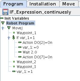
Initially the variable “var_1” is set to 0 –
which means the IF statement is false and will not be executed – until we reach
after Waypoint_3 – then the “var_1” is set to 1 and therefore the IF statement
is true and we be started to be executed.
But in this case we have set the “Check
expression continuously” checked.
What happens now – is that the first few lines
under the IF statement will be executed e.g. the Digital output 2 will go on,
but when we reach “var_1 = 0” in the IF statement, then we actually change the
condition of the IF expression check – which now becomes false – and therefore
the program jumps out of this IF routine already – and the digital output 7
will never go on.
Sometimes we will use Subroutines, but the effect
will be the same.
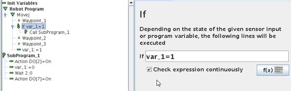
This program will do exactly like the previous
program, but we have used SubProgram method and same thing - the Digital Output
7 will never go on although it says clearly so in the SubProgram, but the IF
expression is already False.
Here we have used a variable to show the
effect, but it could as well have been a Digital Input we have used for the IF
expression check – and the same will happen if the Digital Input state change
while the program are executing the IF program lines – if the IF expression
becomes False during this time – the rest of the program lines will not be executed.
If such state changes right at the moment the IF was true – (but now false)
none of the line in the IF statement are executed.
In a conditional expression you can have
combinations e.g.
IF input_1 = High AND input_2 = Low
Then do something
But make sure you
are using normal mathematically rules – so use of parentheses are a good thing
like this
IF (input_1 =
High) AND (input_2 = Low)
Then do something
However instead
of long mathematically statements – then better have more IF statements.
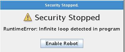
Sometimes when you program – and try to test
run your program you will see an error messages something like this “Infinite
loop detected”. This is because the program is syntax checking your program so
if you have an IF expression for a condition to happen, but never programmed
what to do if the conditions is not present – then you might see this error
messages. The trick is to insert a “dummy” Wait instruction for what to do IF
the expression is not present – just choose a very low value of the Wait e.g.
0.01 Seconds which pass very fast and the program will loop until the IF
expression is true.
Extracting files to the office computer.
After the user program files have been saved
on a USB drive it is very easy to transport them to an office computer for
documentation and backup. Just insert the files into your office computer and
they are there to be viewed.
Aside from the user files the UR controller
also stores the default.intsllation files which are useful if a user program is
transferred to another robot that for some reason had a modified default
installation file. E.g. another IP address. Then it is very easy to reload the
default.installastion file and make the user program run on another robot and.
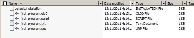
The controller
saves the user program file in three different versions. This is our
“My_first_program” as explained in the “Programming” section of this manual.
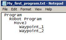
The .txt files
contain a simple description of our user program.
My_first_program.txt
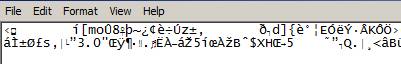
The .urp file is
a binary file that the UR robot use and is not easy readable.
My_first_program.urp
The .script file is our user program as a script file.
My_first_program.script
def
My_first_program():
set_analog_inputrange(0, 0)
set_analog_inputrange(1, 0)
set_analog_outputdomain(0, 0)
set_analog_outputdomain(1, 0)
set_tool_voltage(24)
set_runstate_outputs([])
set_payload(0.0)
set_gravity([0.0, 0.0, 9.82])
while True:
$ 0 "Robot Program"
$ 1 "MoveJ"
$ 2 "Waypoint_1"
movej([-0.7601482324296471,
-1.9284112483400442, 2.4200850009312065, -2.13148960204731, -1.562351390833685,
-0.9523963238633675], a=1.3962634015954636, v=1.0471975511965976)
$ 3 "Waypoint_2"
movej([-0.7601145807261123,
-1.925313457229536, 1.4271208291636501, -1.1406326407517442,
-1.5621569587688118, -0.9518539657810257], a=1.3962634015954636,
v=1.0471975511965976)
end
end
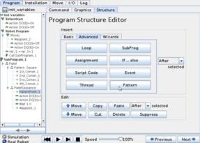
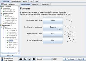
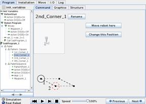
In this case a “Pattern” is chosen in the
Advanced Structure Menu and in the Command screen a “Square” Pattern is chosen.
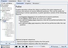
This will create a program entry for a Square
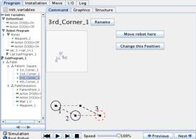
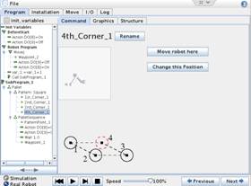
(or Rectangular) Pallet Pattern which consists of the 4 corners of the Pattern
and a program block for the action at each Point in the Square.
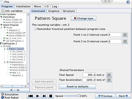
The Pattern
Square the interval count defines the number of position between the
corners. In this case the Square has 8 positions which are arranged 4 by 2. This means the Square (or Rectangular)
does not only consists of the 4 corners, but also the intermediate points
in the Pattern. And individual Speed for the Pattern can
be defined.
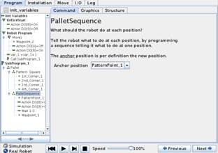
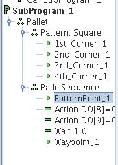
In the “Pallet Sequence” a program can be
created which are to be executed every time the robot reaches a point in the
Pattern.
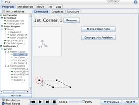
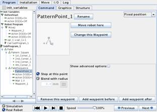
A PatternPoint_1 is like a Waypoint. In this
example the robot has two waypoints and 2 actions and a wait to perform each
time it reaches a one of the 8 positions in the Square Pattern.
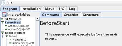
The section of “BeforeStart” in the program
tree is programmed with the normal programming method, but will be executed
only one time before the main program starts.
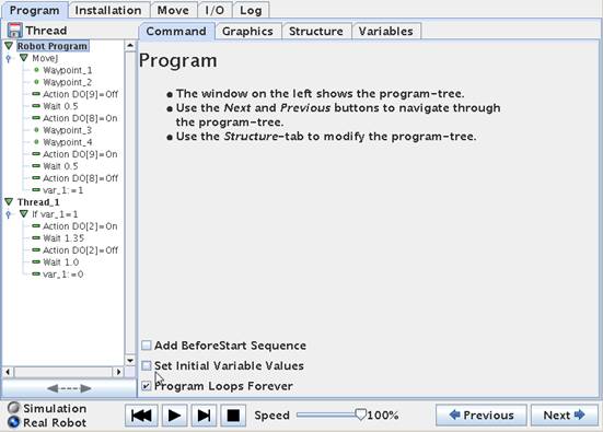
In some cases it is desirable to have a
program sequence which is run before the main program is started and also to
set variables to an initial value and to determine if the program should only
have one passages or loop forever. All these features can be achieved from the
“Robot program” screen. Point the cursor on “Robot Program” in the program tree
structure and a screen like below will appear.
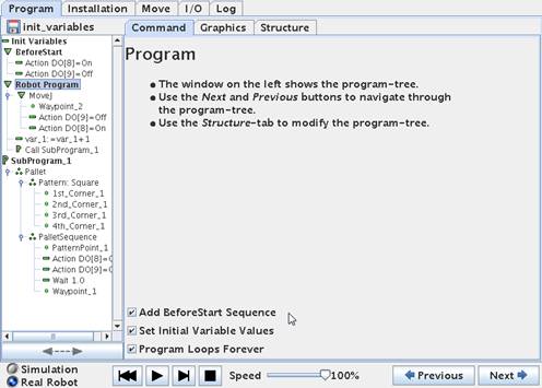
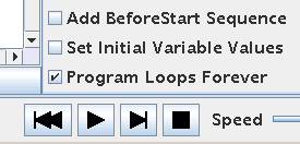
Below in the centre screen is three tick boxes
where “Add Before Start Sequence” and “Set Initial Variables Values can be
activated. And the choice whether the program should have only one run or loop
forever is also set in this screen.
When “Add BeforeStart Sequence” and “Set
Initial Variable Values” are ticked they will be added to the program tree at
the top.
In the Program tree - Point on the “Init Variables”
line and this screen appear.
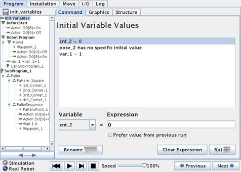
In the centre screen the actual value of the
variables are instantly shown and these variables used in the program can be
set to an initial value desirable for the main program.
The value can also be set to an expression or
to the Value from the last run of the program by ticking the “Preferred value
from previous run”. This is especially useful when using the Pattern templates
for picking or placing items in an array – and therefore continue from the
point from where the robot left from the last program run.
In this case the program comprises of a Pallet
Pattern which has variables for the number of transversal positions to keep
track of the progress besides a user created variable called “var_1”.

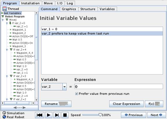
The Init
Variables screen there is a feature called ”Prefer value from previous run”. If
this one is clicked for the intended variable then the robot can remember the
value of the variable form last program run. This is useful to keep track of
positions that changes through the flow of the program.
To control a conveyor that has a function
related to the machine the Robot is tending can by advantage be controlled from
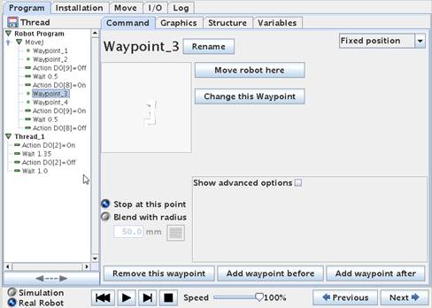
the Robot program. One way to do this is to use the function ”Thread”.
First lest assume we have a program that is
tending a machine. In this small example below Waypoint 1 and 2 is at the
machine and grapping a work piece.
Waypoint 3 and 4 is at the conveyor and at
Waypoint 4 the gripper is released and the work piece is delivered to the
conveyor.
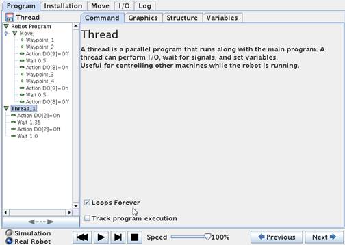
A Thread is a program sequence that is run in
parallel of the main robot program and this can be totally independent of the
robot task – or it can be related to the robot task – up to the programmer to
choose.
This program snippet is at the machine side, but
the conveyor is not moving – and now we want to have the conveyor to move a
notch forward after the robot has delivered a new work piece and then
simultaneously let the robot continue its task while the conveyor is moving
forward.
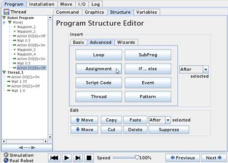
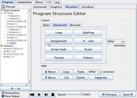
For this function we will use the ”Thread”
which can be found in the ”Structure” menu and under ”Advanced”.
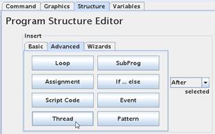
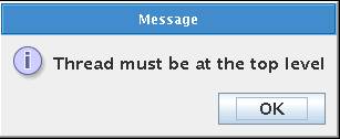
Here we got an error messages because the
Thread has to be at top level. So we have to move the cursor position up and
highlight ”Robot Program” in our program
tree.
And then click ”Thread”.
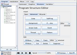
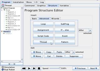
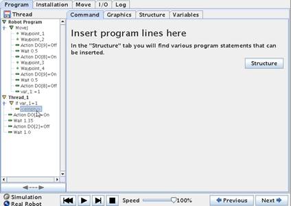
Now a Thread statement has entered our
program. It is shown below our Main program which is slightly confusing because
we got told before that it should be at top level. However it is more correct
to say that the Thread is at the side of our Main program because it twill run
in parallel with our main program.
The Thread can be programmed exactly in the
same way as our main program – and we can even have Waypoints inside the
Thread, but then make sure that is intended in relation to the main program –
otherwise the Waypoint action inside the Thread might conflict with the Waypoint
action in the Main program (The robot cannot be a two positions at the same
time).
We want the conveyor to go on for a short
while – and the off the conveyor again. An example of this function is shown
under the Thread above.
This example assumes that the conveyor is
controlled by out put DO2. There is a Wait in between the ON and OFF statements
which is our conveyor run time.
After the OFF statement there is another Wait
because otherwise the conveyor would go ON immediately we stopped it – and the
result would be a continuously running conveyor.
Although this will run the conveyor in 1.35
seconds in this case – it is still independent of the robot action – which is
not our intention – so we need a little more programming.
We need to synchronize the Thread with the
Main Program and there are many ways to do it, but one way is setting a
variable in the main program and then checking on this variable in the thread.
The plan is to set a variable at a certain
value in the main program at the time we want the conveyor to start – this is a
flag to the Thread program.
We have to identify in the main program –
where is it we want the conveyor to move forward ?. In this case it is after
the robot has delivered the work piece to the conveyor – which is at Waypoint 4
and after we have released the work piece.
So we put the cursor there and go to
”Structure” – ”Advanced” and choose ”Assignment”.
This will bring a ”=” (equal) sign into the
program. We need to define the ”Assignment”.
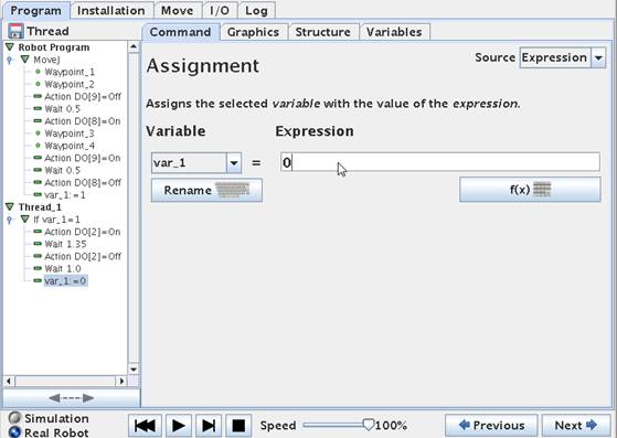
Click on
”Command” to get the property screen for ”Assignment”.
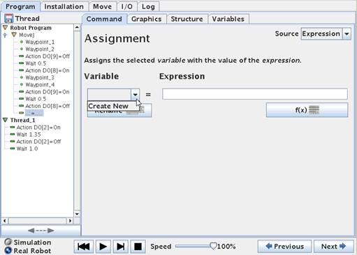
This is our first variable so we have to
create it. Click on ”Create New”.
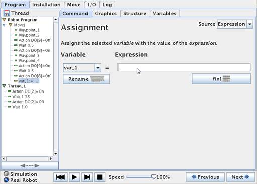
The Robot will automatically name it ”var_1”,
but you can rename to your own preferred name, but often for trouble shooting
and discussion with colleagues it is better to leave as the original name.
On the right hand side is an ”Expression”
field because we can assign the variable a fixed value or a value base don an
expression – maybe base don the previous value of the variable for example to
make counters.
But in our case the variable is just a Flag to
tell us where we are in the program sequence – so we just give it the value of
”1”.
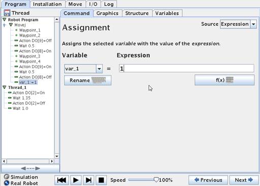
Note how the ”var_1” in the main program has
been assigned to the value of 1.
When the ”var_1” variable is 1 - it tells us that the main program has reach
the point when the work piece has been delivered to the conveyor. That’s great
because that’s exactly when we want the conveyor to start.
So we will make the Thread dependant on this
”var_1” variable.
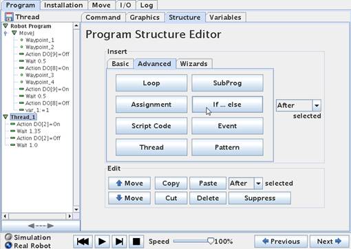
Insert an IF statement into the Thread.
Define the IF
statement by clicking on the formula button.
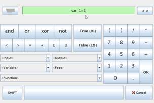
This will bring up a screen where we can
choose the ”var_1” variable and choose to design our expression as var_1=1.
This means that only IF var_1 = 1 then we will execute the program line below
the IF statement.
Make sure the
”Check expression continuously” is not ticked. If this is checked the robot
will check IF ”var_1”=1 is true also during the Thread execution. This means
that if the ”var_1” becomes 0 during the Thread execution then the rest of the
program lines inside the IF will not be executed. This can lead to unintended
function if not handled correct. In our case we need to set the ”var_1” to 0
inside the Thread and if we do that on top of the program lines below the IF –
then the rest of the IF program lines will not be executed.
Now we have a little Editing work to do –
because what we actually want the lines we originally had in the Thread to be
under the IF statement (otherwise the lines will be executed no matter what is
the result if the IF expression.
So we need to move those 4 lines up under the
IF by using Cut/Paste or create them again.
Notice how all 4 lines now is directly under
the IF statement.
But we only want the conveyor to run one time
– every time it is triggered. So we have to make sure our IF statement becomes
False next time the program check the IF expression.
Therefore we insert a ”Assignment” in the
Thread where we zero the ”var_1” variable so it becomes False for the IF check.
We set the ”var_1” variable to 0 in the
property screen for the variable.
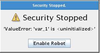
If you get this error messages it is because
we need to tell the Robot – what should the variable ”var_1” be when we start
the program. This is uncertain for the robot if we have not explicit set the
variable before the program execution.
So we have to put the cursor up on top where
it says ”Robot Program”
And then tick ”Set Initial Variable Values”.
This will insert a line op top of the program
called ”Init Variables”.
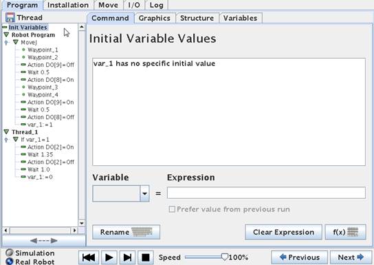
The Init Variables screen shows that the
”var_1” has no Initial Value.
Below the messages box is a function to set
variables.
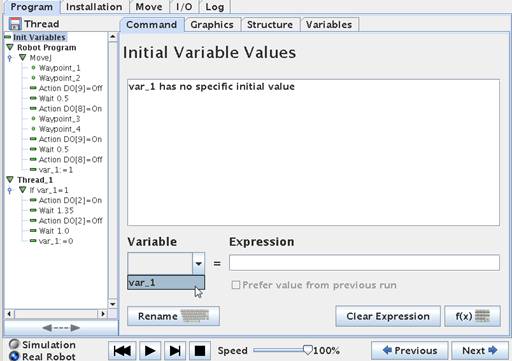
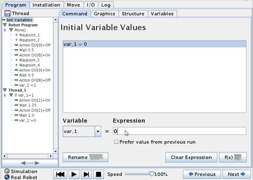
Choose ”var_1” and insert 0 in the Expression
field.
If you get this error messages is because the
robot does not like to be caught in an Infinite loop. In this case the Thread
program might be Infinite if the ”var_1” never change.
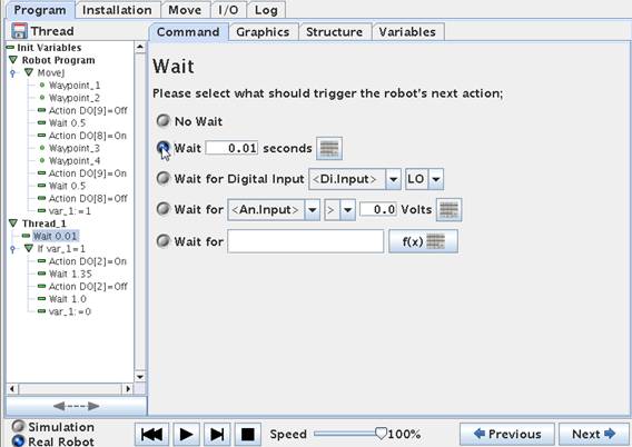
So we do the trick by inserting a small and
very short ”Wait” and put it at a very low value e.g. 0.01 seconds.
This is done before the IF statement in the
Thread – so the Thread has something else to do if ”var-1” is not 1. (In this
case – to wait 0.01 seconds).
The entire program looks like this below.
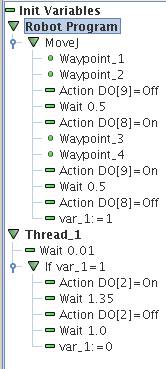
This small program is working and the logic is
like this.
Before the program starts the variable ”var_1”
is set to 0 in the Init Variables statement.
The Robot Program and the Thread is run
simultaneously, but because the ”var_1” equals 0 the IF statement in the Thread
is False at this moment so the conveyor is stopped.
The main program start moving the robot from
Waypoint 1 to waypoint 2 – then the DO8 goes ON which could be the gripper
closing (In my case I have set the DO9 to go off because of the configuration
of the valves I use to open and close the gripper).
The robot move through Waypoint 3 and 4 –
where I imagine the robot is now at the conveyor position ready to deliver the
item – so the out put DO8 go off and DO9 go on. This will deliver the item onto
the conveyor. Right after this I set the variable ”var_1” to the value ”1”
because I want to flag to the Thread that the conveyor can move.
In the Thread the IF statement now see the
”var_1” as ”1” and therefore will perform our code inside the IF statement
–which is to Start the conveyor DO2 is set to ON. We wait 1.35 seconds and turn
the conveyor OFF again. And then the ”var_1” is set to ”0” because when the IF
statement is checked again it is not False and the conveyor remains
stopped - as we wish.
While the Thread is doing this and the
conveyor is moving – the robot is long moved on in its cycle in the main
program.
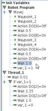
If a small Wait statement is inserted before the
”var_1” = 1 in the main program the conveyor has a delay before it starts and
let the robot gripper get out of the way.
If you wish to place the work pieces in rows
on the conveyor – maybe 2 rows or 4 rows etc.
So in this example I will show 4 rows.
Maybe in a pattern something like this.
Basket
↑
O O
O O
O O
O O
O O
O O
Robot
The sequence the work pieces has been put on
the conveyor is like this
Basket
↑
1 2
3 4
1 2
3 4
1 2
3 4
Robot
This means the Conveyor only have to move a
notch forward in between 2 and 3. And again in between 4 and 1.
A way to program this is just to use variables
and IF statements to keep track of the sequences of placing work pieces in this
pattern in the Main program.
And then let the Thread take care of the
moving the conveyor a notch forward. The Thread does actually not need to know
the sequence of placing work pieces – the Thread just ON/OFF the conveyor
according to the timing set inside the Thread.
So the Thread will remain like in the previously
example.
(There are many different ways to do this – as
many there are creative programmers).
So far there is only
one Waypoint for delivering the work piece because it is always delivered at
the same position on the conveyor. In previous chapter this is Waypoint 4 that
is the position for delivering the work piece.
Now in this example we need 4 different
waypoints for delivering the work piece on the conveyor because position 1 – 2
– 3 – and 4 are different. To keep track of the delivery position we can use
another variable.
Let’s get do some programming.
The first part of the program is almost like
before until we reach the point where we have to deliver the work piece onto
the conveyor.
However on top of the main program there has
been an IF statement inserted which is to initialize our position counter. The
position counter is a new variable called ”var_2”.
In the Init Variables block we set the ”var_2”
to 0. So first time we run the program – the variable will be 0 and thereby we
know this is the first run and we can change the value to 1 so we can place the
first work piece at position 1.
If we use the function to store values of this
variable in between runs – then we can achieve that the robot can remember
which position on the conveyor is the next position – this will be explained
later.
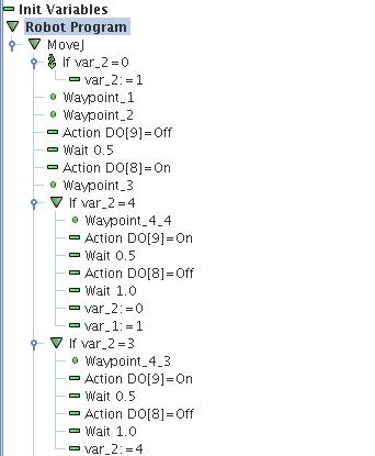
Since we have 4 different positions for the
robot to deliver the work piece to - we have to create 4 waypoint for this
position across the conveyor belt. These 4 waypoint will be in line across the
conveyor belt because it is the moving forward of the belt that provides the
zigzag pattern. So we will put the first at position 1 and then position 2 –
move the conveyor a little forward – then put at position 3 and finally at
position 4 and move the belt a little forward.
In the program I
now call the waypoints 4_1, 4_2, 4_3, 4_4 just to illustrate that it is
Waypoint 4 we are working with. There can be more Waypoints at these position e.g.
an up and down and back up again for nice placement of the part.
So before programming any further we will
define the Waypoint_4_1 ,
Waypoint_4_2 , Waypoint_4_3 , Waypoint_4_4 where we want them to be at
the conveyor.
After the 4 Waypoints have been defined we
will introduce 4 IF statements because we need to check where the next work
piece have to be placed.
We introduced the variable ”var_2” for this
purpose.
The ”var_2” can in this case have 5 different
values i.e. 0, 1, 2, 3 and 4.
The value 0 is to tell that we start all over
again.
At the first run the ”var_2” will have the
value 0 – which is very quickly changed to 1 in the beginning of the main
program. So when we come down to the IF statements the value of ”var_2” is 1.
And the program under ”IF var_2 = 1” will be executed – which is to go over to
Waypoint_4_1 and deliver the part.
When the part has been delivered to
Waypoint_4_1 the variable ”var_2” is set to 2 – to show the robot program
that we have already been at position
one and the next position in line is position 2.
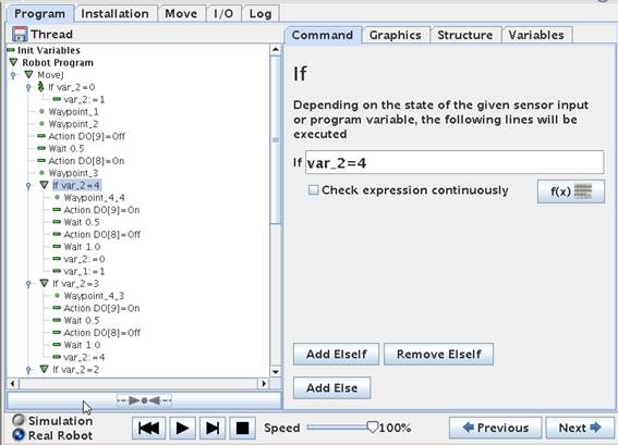
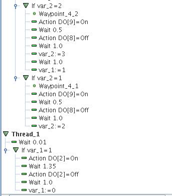
Notice how the IF statement of ”IF var_2 = 4”
is on top and going down to ”IF var_2 =
4”. The reason for that is because we set the ”var_2” variable inside the IF
statement to the next value – and if we had the ”IF var_2 = 1” on top down to
”IF var_2 = 4” – then all IF would be executed in a row because the change of
”var_2” will make it true for the next IF. That’s why they are turned upside
down.
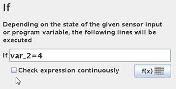
Leave the ”Check expression continuously” at
each of these 4 IF statements in the main program unchecked.
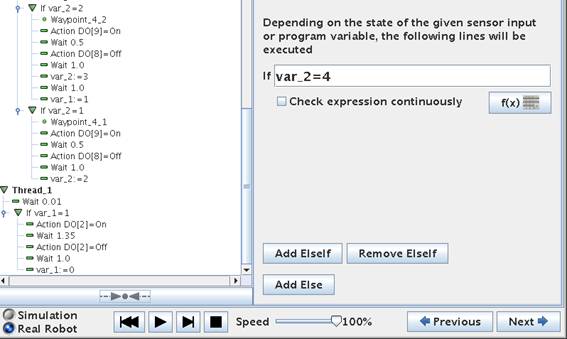
Since we only need to conveyor to move forward
after position 2 and after position 4 the assignment of ”var_1” is only done
inside the IF statement for Waypoint_4_2 and Waypoint_4_4.
So the IF statement inside the Thread is only
true after the robot has delivered to Waypoint_4_2 and Waypoint_4_4.
The entire
program looks like this.
Here comes a
beautiful function.
So far the robot program will start at
position 1 (Waypoint_4_1) every time we start up the Robot program – also is
this was after a safety stop.
But in the Init Variables screen there is a
feature called ”Prefer value from previous run”. If this one is clicked for the
intended variable then the robot can remember which position is next to be
delivered to on the conveyor so we do not stack to work piece on top of each
other or leaves any location unoccupied.
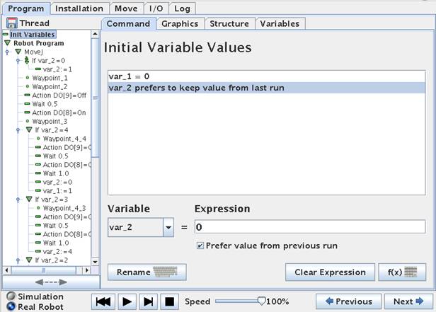
So far we have used the touch screen teaching
pendant on the Universal-Robot to make our robot programs which is very
convenient and easy to build up programs.
But sometimes it can be desirable to be able
to make the robot program on a host computer and just communicating and sending
commands from the host computer or PC via an Ethernet socket connection
directly to the robot motion and action control without using the teaching
pendant. For example if the robot is part of a big complex installation where all
equipment are controlled from the host computer or PC.
Another advantage by doing this is that the
program can be further developed, edited and tidy up while the robot is running
production. Then when there is a break in the production the new modified
program can be activated and control the robot right away (provided the
programmer did not make any programming errors in the new version).
The differences in using the teaching pendant
and the remote scripting method is that when editing with the teaching pendant
the program execution has to be stopped while editing and thereby interrupt the
actual production whereas editing in the host application can be done aside
from the running version and thereby not disturb the production.
Another advantage is that the host application
programmer can make new functions and features by himself and basically create
a complete new user interface and functionalities to the robot and handling of
his data and interfacing with even other computer systems to his creativity
abilities.
The Universal-Robot offers such possibilities
to make remote script programming with its build in script interpreter. The
choice of programming environment on the host computer is up to the programmer
and typically programming languages such as C++, Java, Visual Basic, and Python
or similar is the choice, but even Notepads can be used as an editor.
But before jumping into the remote script
programming there is also an alternative script programming method provide by
the teaching pendant as well which is also very useful. With this method it is
possible to Import Script statements or whole Script files into the robot
program created by the teaching pendant – so this method is something in
between using only the teaching pendants program objects and the fully remote
Script programming. This method will be explained first.
It is also important to mention the separate
document and manual for Universal-Robot script programming called “scriptmanual_enx.x”
where the commands with their parameters are explained.
In this method of script programming you still
need the teaching pendant, but this function is very helpful and makes it
possible to edit part or entire program on another computer while the robot is
running production.
This function can be used extensive script
programming, but also just as a method to manipulate variables, input/output
states and especially timers. This makes the programming very elegant i.e. the
program tree is the overall pattern and flow of the program whereas things that
can change such as variables I/O and timers are kept in separate blocks. In
this way the commissioning and adjustment can be done in these blocks without
touching the program flow.
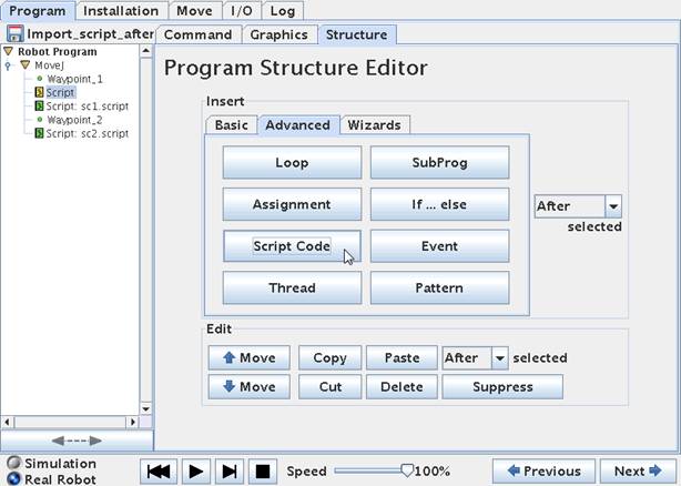
In the Advanced program menu under Structure
section the Script Code object is located. This object will insert at “Script:”
entry into the program. Note it is still yellow which means we have to define
it.
To define the Script entry in the program –
point on the Script line to define and choose “Command” on top of the menus.
However before we
proceed with the programming we need to prepare our Script file – otherwise
there is nothing to load so let’s step a little back to the point where we have
no Script entries in the program tree and just two simple Waypoints.
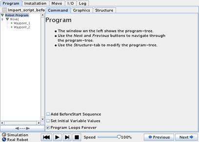
I am planning to change 2 outputs in between
the two Waypoints and after the last Waypoint before the program goes back to
Waypoint 1. And I need a delay in between the change of the 2 outputs – note
the second delay is 2 seconds whereas the first is 1 second.
This could also be done by using the
traditional teaching pendant method and it would look like below program.
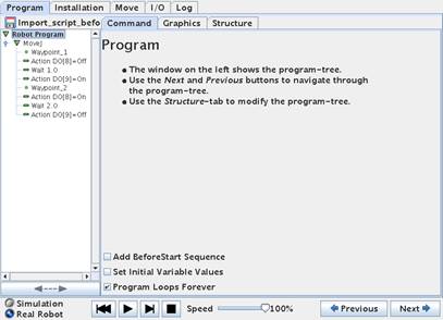
But in this case we want to use the Script
method so we have a separate Script file with our variables for later
adjustment opportunity while the robot is running production.
So before we go any further we only have a
small program with 2 waypoints.
Now we need to prepare the separate Script
file. The format of the Script statements can be studied in the Script manual,
but a very useful method to learn about the format of a Script language is to
open a Script file the robot already have provided from previous created
program. Remember the robot creates three files every time a program file is
saved – a x.urp file which is the robots main program file – a x.txt file which
is a very simple text file to illustrate the program flow and a x.script file
which is the actual program in script format. Try and open such an x.script file
in a simple editor e.g. a Notepad and study the contents.
For example our first program looked like this
in script format:
My_first_program.script
def
My_first_program():
set_analog_inputrange(0, 0)
set_analog_inputrange(1, 0)
set_analog_outputdomain(0, 0)
set_analog_outputdomain(1, 0)
set_tool_voltage(24)
set_runstate_outputs([])
set_payload(0.0)
set_gravity([0.0, 0.0, 9.82])
while True:
$ 0 "Robot Program"
$ 1 "MoveJ"
$ 2 "Waypoint_1"
movej([-0.7601482324296471, -1.9284112483400442,
2.4200850009312065, -2.13148960204731, -1.562351390833685,
-0.9523963238633675], a=1.3962634015954636, v=1.0471975511965976)
$ 3 "Waypoint_2"
movej([-0.7601145807261123,
-1.925313457229536, 1.4271208291636501, -1.1406326407517442,
-1.5621569587688118, -0.9518539657810257], a=1.3962634015954636,
v=1.0471975511965976)
end
end
Don’t dwell too much into the details at this
stage of this script file and may just study a single line statement e.g. the “set_tool_voltage(24)” which sets the Voltage on the tool to 24
Volt and compare to the explanation in the “scriptmanual_enx.x” document.
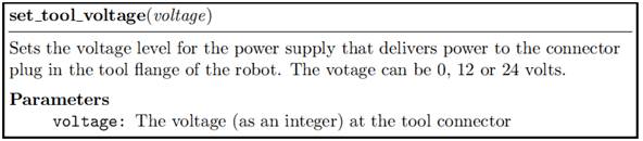
Note that in this case the robot has wrapped
the Script code around with some initial definitions that you do not see in the
tree structure, but that’s default robot settings and also comments like “$ 2 "Waypoint_1"” – this you might or might not need in
your Script file depending on your complexity of your Script program and also
because we are inserting Script code into a part of a already existing robot
program and therefore some of these wrappings will be duplicated and cause
program errors – so in this first simple case we do not need it.
Study also the long “movej(xx, xx, xx, …………,
v= xx) which is actual positions of the waypoints. The meaning of the values
will be explained later section
In our case we just need two script files
because we need to insert Script code at to different locations in the program
i.e. in between the Waypoints and after the last Waypoint – and we need two
files because they need different contents because we swap the status of the
outputs.
Some we will now prepare the Script files on a
PC computer and we just use a simple editor such as Notepad to create these two
files.
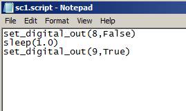
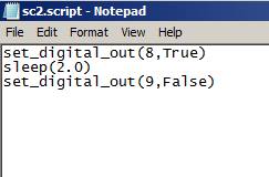
Note that the two outputs have swooped states
and the delay has increased from 1 to 2 seconds. Also note the two files has
different names i.e. sc1.script and sc2.script.
Also note how the “Wait 1.0” functions is now
called “Sleep(1.0)” which is in line with standard Script language.
So now instead of programming these functions
in the program tree we want to import these files instead.
Now we can proceed to insert a Script:
statement into the program tree by picking it from the advanced program object
menu and it comes into the program as yellow because so far it is undefined.
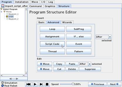
Point on the “Script:” statement and choose
“Command” screen. In this screen the Script function is defined. On the right
hand side the amount of script commands are chosen i.e. only one line of script
code or from a separate file containing maybe several script commands.
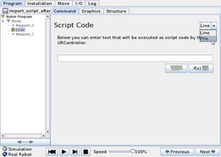
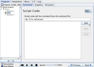
In this case we choose file because understand
file will also explain a single line – and the right screen appears.
So far no file has been chosen – hence there are
no script statements. Choose “Edit”.
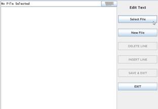

Then choose “Select File” which will bring you
to the file menu where you can navigate to your file destination of your
prepared Script program block. Then choose your intended Script file and choose
Open – in this case the sc1.script file we have prepared and choose “Open”.
This will open your Script file. Choose “Save
& Exit” which will complete you’re “Script:” statement in the program tree
and therefore turn green.
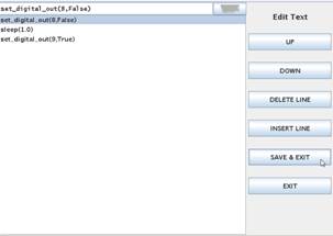
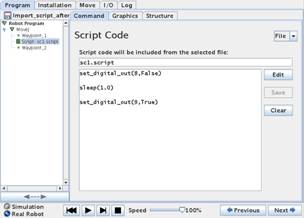
Note how the contents of the Script file now
have entered into our program under the Script: statement.
Now follow the exact way to insert a second
“Script” statement under Waypoint_2, but this time import the script file
“sc2.script” instead.
Then your program should look like this.
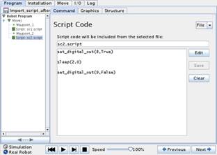
Now try to test run your program which behave exactly
like if the outputs and wait has been made in the tree structure.
Save the file which of cause will create three
new files x.urp, x.txt and x.script which now has the entire program inside
including the Script files interpreted by the Robot.
def
Import_script_after():
set_analog_inputrange(0, 0)
set_analog_inputrange(1, 0)
set_analog_outputdomain(0, 0)
set_analog_outputdomain(1, 0)
set_tool_voltage(24)
set_runstate_outputs([])
set_payload(0.0)
set_gravity([0.0, 0.0, 9.82])
while True:
$ 0 "Robot Program"
$ 1 "MoveJ"
$ 2 "Waypoint_1"
movej([-0.5263706597088378,
-1.8182878349727298, -1.8120234982472114, -1.3619128328552264,
3.214885380931556, -0.27251695975573664], a=1.3962634015954636,
v=1.0471975511965976)
set_digital_out(8,False)
sleep(1.0)
set_digital_out(9,True)
$ 4 "Waypoint_2"
movej([-0.8560998108900053,
-1.7976119215251396, -1.7847397963745542, -1.410065160905723,
3.2146832909469674, -0.27251695975573664], a=1.3962634015954636,
v=1.0471975511965976)
set_digital_out(8,True)
sleep(2.0)
set_digital_out(9,False)
end
end
Note how the content of our two script files
has been inserted to the program (marked with yellow). The big advantage now is
that we still have our two script files we can edit with an editor on another
computer and make adjustments to our variables e.g. if we want to change output
or change timer values it can be done while the robot is running production and
then when there is a break be loaded into the robot program which can immediately
be started.
It is possible to have the entire program as a
script file and import in this way – so the tree structure will only have one
statement – a Script: statement where the entire program is in a script file
and thereby loaded into the robot. But in such case some of the wrappings and
comments has to be removed from the script file format the robot create by
itself in order to avoid double definitions.
The previous chapter used the “Script:”
function available in the teaching pendant to import blocks of Script code or
entire program into the robot and run from the teaching pendant.
In this chapter we will focus on making a
script that entirely control the robot remotely from a host computer by Script
programming.
The format is the same as in previous chapter
and as documented in the Script manual, but since we are not using the teaching
pendant we need to send the Script file to the Robot control through an already
prepared open port on the Robot which is TCP port 30002.
In this case we are using the program language
Python and the Python environment to communicate with the Robot. The Script
file can still be edited in a Notepad.
The first program example is just to
illustrate how to send a script file through via the Ethernet to the TCP port
300002 on the robot.
In this case the robot has already been
configured to IP address 192.168.0.9 and our host must be in the same subnet
e.g. defined as 255.255.255.0
The first Program 1 just turns digital output
number 2 ON and the robot does not move at all and the program looks like this.
#
Echo client program
import
socket
HOST
= "192.168.0.9" # The remote
host
PORT
= 30002 # The same port as
used by the server
s
= socket.socket(socket.AF_INET, socket.SOCK_STREAM)
s.connect((HOST,
PORT))
s.send
("set_digital_out(2,True)" + "\n")
data
= s.recv(1024)
s.close()
print
("Received", repr(data))
The program is run from the host computer and
will only have one passage because there is no loop in the program.
The library “socket” in imported into the
program so the Socket connection is available. The “Host” in this case is the
Robot and “PORT” is the open port on the Robot that listens for Script code.
Then the Script code necessary to connect and
send on the Socket. The “s.send” command send that actual script code for the
robot to execute which in the case is ("set_digital_out(2,True)” Which is like previous chapter. The + "\n") at the end of the line is a linefeed
because the Robot need a linefeed after each command. The Socket connection
needs to be closed again with the s.close() command. The print ("Received", repr(data)) command prints the output from the robot on the Host
or PC monitor – in this case acknowledgement code.
The second Program 2 is similar and just turn
digital out number 2 OFF again and the robot does not move at all.
#
Echo client program
import
socket
HOST
= "192.168.0.9" # The remote
host
PORT
= 30002 # The same port as
used by the server
s
= socket.socket(socket.AF_INET, socket.SOCK_STREAM)
s.connect((HOST,
PORT))
s.send
("set_digital_out(2,False)" + "\n")
data
= s.recv(1024)
s.close()
print
("Received", repr(data))
#
Echo client program
import
socket
import
time
HOST
= "192.168.0.9" # The remote
host
PORT
= 30002 # The same port as
used by the server
print
"Starting Program"
count
= 0
while
(count < 1):
s = socket.socket(socket.AF_INET,
socket.SOCK_STREAM)
s.connect((HOST, PORT))
time.sleep(0.05)
s.send ("set_digital_out(2,True)"
+ "\n")
time.sleep(0.1)
print "0.2 seconds are up already"
s.send ("set_digital_out(7,True)"
+ "\n")
time.sleep(2)
s.send ("movej([-0.5405182705025187,
-2.350330184112267, -1.316631037266588, -2.2775736604458237,
3.3528323423665642, -1.2291967454894914], a=1.3962634015954636,
v=1.0471975511965976)" + "\n")
time.sleep(2)
s.send ("movej([-0.7203210737806529,
-1.82796919039503, -1.8248107684866093, -1.3401161163439792, 3.214294414832996,
-0.2722986670990757], a=1.3962634015954636, v=1.0471975511965976)" +
"\n")
time.sleep(2)
s.send ("movej([-0.5405182705025187,
-2.350330184112267, -1.316631037266588, -2.2775736604458237,
3.3528323423665642, -1.2291967454894914], a=1.3962634015954636,
v=1.0471975511965976)" + "\n")
time.sleep(2)
s.send ("movej([-0.720213311630304,
-1.8280069071476523, -1.8247689994680725, -1.3396385689499288,
3.215063610324356, -0.27251695975573664], a=1.3962634015954636,
v=1.0471975511965976)" + "\n")
time.sleep(2)
s.send ("movej([-0.540537125683036,
-2.2018732555807086, -1.0986348160112505, -2.6437150406384227,
3.352864759694935, -1.2294883935868013], a=1.3962634015954636,
v=1.0471975511965976)" + "\n")
time.sleep(2)
s.send ("movej([-0.5405182705025187,
-2.350330184112267, -1.316631037266588, -2.2775736604458237,
3.3528323423665642, -1.2291967454894914], a=1.3962634015954636,
v=1.0471975511965976)" + "\n")
time.sleep(2)
s.send ("movej([-0.7203210737806529,
-1.570750000000000, -1.570750000000000, -1.3401161163439792,
3.2142944148329960, -0.2722986670990757], t=4.0000000000000000, r=0.0000000000000000)"
+ "\n")
time.sleep(4)
s.send
("set_digital_out(2,False)" + "\n")
time.sleep(0.05)
print "0.2 seconds are up
already"
s.send
("set_digital_out(7,False)" + "\n")
time.sleep(1)
count = count + 1
print "The count is:", count
time.sleep(1)
data = s.recv(1024)
s.close()
print ("Received", repr(data))
print
"Program finish"
******************************************************************************************************************************************************************************************************************************************************
#
Echo client program
import
socket (Import the library for Socket
connections)
import
time (Import the library for Time
function)
HOST
= "192.168.0.9" # The remote
host (IP address of the robot)
PORT
= 30002 # The same port as
used by the server (The port socket open on the
robot for script programming)
print
"Starting Program" (This is printed on the PC
Computer from where the script program is run).
count
= 0 (set the variable “count” to
value 0)
while
(count < 1): (Loop unitl count is smaller
than 1, but not 0)
s = socket.socket(socket.AF_INET,
socket.SOCK_STREAM) (All line that is indented under
the While statement is executed in the loop).
s.connect((HOST, PORT)) (Connect to the robot port)
time.sleep(0.05) (Wait 0.05 seconds because the
robot communication speed is 125 Hz = 0.008 seconds)
s.send ("set_digital_out(2,True)"
+ "\n") (Set digital output 2 high
)True))
time.sleep(0.1) (Wait for communication speed)
print "0.2 seconds are up
already" (Print messages on PC Computer
screen)
s.send ("set_digital_out(7,True)"
+ "\n")
time.sleep(2)
s.send ("movej([-0.5405182705025187,
-2.350330184112267, -1.316631037266588, -2.2775736604458237,
3.3528323423665642, -1.2291967454894914], a=1.3962634015954636,
v=1.0471975511965976)" + "\n")
a = joint accleration v = joint speed
time.sleep(2) (Wait for robot to move to
Waypoint)
s.send ("movej([-0.7203210737806529,
-1.82796919039503, -1.8248107684866093, -1.3401161163439792, 3.214294414832996,
-0.2722986670990757], a=1.3962634015954636, v=1.0471975511965976)" +
"\n")
time.sleep(2)
s.send ("movej([-0.5405182705025187,
-2.350330184112267, -1.316631037266588, -2.2775736604458237,
3.3528323423665642, -1.2291967454894914], a=1.3962634015954636,
v=1.0471975511965976)" + "\n")
time.sleep(2)
s.send ("movej([-0.720213311630304,
-1.8280069071476523, -1.8247689994680725, -1.3396385689499288,
3.215063610324356, -0.27251695975573664], a=1.3962634015954636,
v=1.0471975511965976)" + "\n")
time.sleep(2)
s.send ("movej([-0.540537125683036,
-2.2018732555807086, -1.0986348160112505, -2.6437150406384227,
3.352864759694935, -1.2294883935868013], a=1.3962634015954636,
v=1.0471975511965976)" + "\n")
time.sleep(2)
s.send ("movej([-0.5405182705025187,
-2.350330184112267, -1.316631037266588, -2.2775736604458237, 3.3528323423665642,
-1.2291967454894914], a=1.3962634015954636, v=1.0471975511965976)" +
"\n")
time.sleep(2)
s.send ("movej([-0.7203210737806529, -1.570750000000000,
-1.570750000000000, -1.3401161163439792, 3.2142944148329960,
-0.2722986670990757], t=4.0000000000000000, r=0.0000000000000000)" +
"\n")
(Second joint at -90 deg
t = (time to reach this r = (Blend
radius is set to 0) .
waypoint
is 4 sec) .
(In robot Move Screen the jopint positions expressed in
degrees i.e. -360 to 360 degrees. Here the joint positions are expressed as
radians where -360 = -6.283, -180= -3.14,
-190 = -1.57075, 0
= 0, 90 = 1.57075, 180 = 3.1415, 360 = 6.283)
time.sleep(4) (Program waits 4 second because it
takes 4 seonds for the robot to move to the waypoint).
s.send
("set_digital_out(2,False)" + "\n")
time.sleep(0.05)
print "0.2 seconds are up
already"
s.send
("set_digital_out(7,False)" + "\n")
time.sleep(1)
count = count + 1
print
"The count is:", count
time.sleep(1)
data = s.recv(1024)
s.close()
print ("Received", repr(data))
print
"Program finish"
The Features screen in the ”Installation”
screen is a option to define the robots movement to user defined relative
points.
These points can be used in the ”Move” screen
as from where the robot should move relative to when using the Arrow keys in
the ”Move” screen.
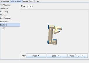
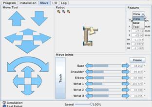
Before we define
any new relative points or patterns lets checkout the ”Move” screen.
On the top right
hand corner is a Feature control. And the robot has already three predefined
relative points i.e. ”View”, ”Base” and ”Tool”. By default the View is active.
To explain how the Robot move relative to this
point the ”Up” and ”Down” arrow keys are used because they are easy to
understand.
If the robot is mounted like on a table top
mounting the ”View” feature relative is like you see (observe - view) the robot
and when pressing the ”Up” the robot moves straight up and when pressing ”Down”
the robot moves straight down. Choosing ”Base” feature will be the same in this
case if the Robot is mounted as table top mounting, but different if the Robot
is mounted on Wall or Ceiling or in an angle.
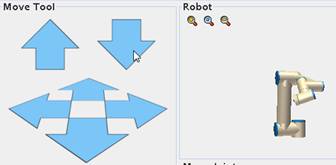
If the Feature is
changed to ”Tool” the ”Up” and ”Down” arrows move in the Tool heads core axis.
Try and set the tool head in an angle relative to the horizon and press the
”Up” and ”Down” arrows – and observe how the robot now moves in the Tool head
axis which is not straight up and down if the head is already in an angle.
Observe the Graphics on this screen which
shows the tool head like it is vertical to the horizon, but a closer look will
reveal that the base is in an angle and therefore the graphics will show the
robot head go up and down, but by observing the robot the head moves in the
tool head score plane. This is useful in programming the robot if we are moving
relative to an object.
We can also define our own relative points –
or line or plane. Go back to the Feature ´s in the Installation screen.
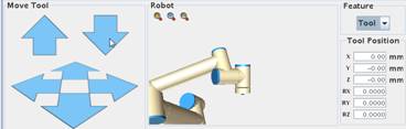
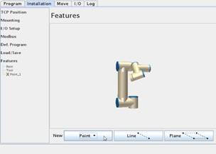
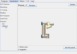
Notice under features is already Base and Tool
which are the build in default relative point.
Below press ”Point” which will insert a red
”X” under Base called Point_1. It is red because it is not yet defined. Point
on the red ”X” and pres sit which brings this screen from where you can define
(Set this point) like setting a waypoint.
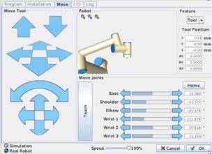
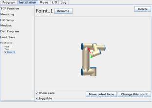
When the relative point has been set (can be a
corner of a table or a machine part e.g. a CNC chuck) then press ”OK”.
Now the Point_1 relative point has been
defined.
Since we are in
this screen then Point at Features again and set a Line and Plane relative
points.
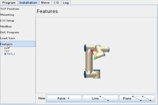
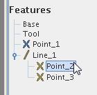
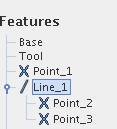
For ”Line” you
need to define the two end points of the line.
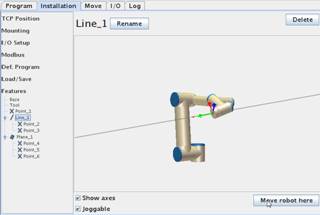
For ”Plane” you
need to set three point of the Plane. Choose the ”Show axes” so you can see the
axis on the graphics and Tick the ”Joggable” to make it active in the ”Move”
screen.
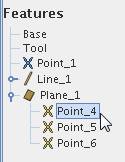
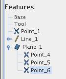
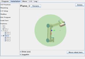
Go back to the
”Move” screen and notice how these three relative points, Line, Plane has been
added the ”Feature” menu. Try to choose each of the new relative objects.
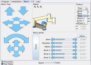
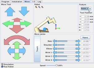
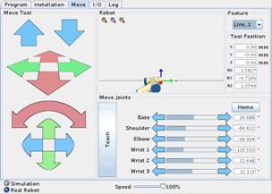
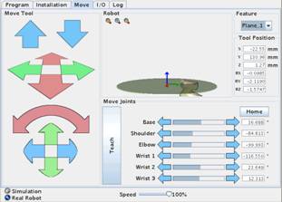
Try and go back
to the ”Feature” screen in the installation screen.
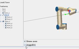
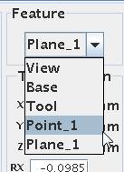
Try and un-tick
the ”Joggable”. Go
back to the ”Move” screen.
Notice how the
”Line_1” is now missing i.e. that ”Joggable will determine if we have it
available in the Feature menu. This Feature is useful when programming the
robot and the waypoints are define relative to an object, Line or Plane and it
is easier to position the robot.
Digital Outputs on
tool head are Open collector type. Open collector means that the outputs are
implemented to ”sink” and we can say they are ”Active low” because connecting
an actuator can be done by applying the supply voltage at the ”far” end of the
actuator connections and the other connection to the output terminal - and then
when the output is driven low by the programmer – the external device turns on.
If you prefer to
have an ”Active high” output – it is also possible – then just apply a ”pull up
resistor”. So now the ”far” end of the external device is connected to GND and
the other end is connected to the output and a pull up resistor. The pull up
resistor is connected to the supply voltage. Now when the output is driven
”high” by the programmer the external device turns on.
Open collector is
actually an advantage because it gives the implementation more choices.
The method of "Potential Free"
signal exchange is very elegant because we don’t mind if one machine is 12 Volt
and the other is 24 volt - we just detect when the contact set open and close
with our "own" power on the machine we need the information.
This principle of Potential Free handshake is
also advisable to use for the normal Start and Idle signals i.e. the Start
signal on the CNC machine should just be a dry contact controlled by a relay on
an output on the Robot. And the Idle signal should just be a dry contact (controlled
by a relay - e.g. via the beacon) on the CNC machine.
That’s "Potential Free" signal
exchange and the Power Supplies on the two machines is not connected at all,
but we still have handshake through the dry contacts.
If the number of I/O interface ports on the
controller board and tool head is not enough then it is possible to extend by
installing external MODBUS nodes.
They are connected to the UR controller via
the Ethernet and the UR controller programming method is prepared to read and
set these external I/O signals as they were a part of the integrated
controller.
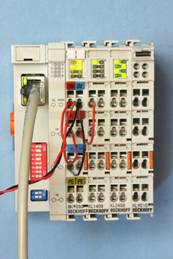
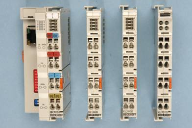
Example of Modbus
configuration using BK 9050, KL 1408, KL 2408 and KL 9010 Modbus modules.
BK 9050 = Modbus
Controller with Ethernet port for IP configuration.
KL 1408 = Modbus
8 port input module.
KL 2408 = Modbus
8 port output module.
KL 9010 = Modbus
End terminator.
The IP address of the Modbus node has to be
defined in the Robot configuration.
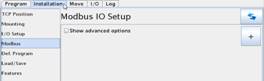
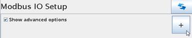
Tick the “Show advanced options” and press the
“+” sign.
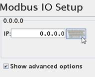
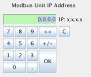
In our case the Modbus node has been setup for
the IP address of 192.168.0.10 and therefore we have to define this for the
Robot.
Press the
Keyboard icon next to the IP: address field.
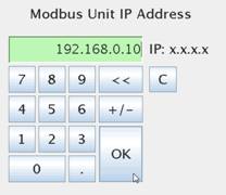
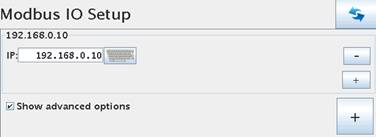
Key in the IP
address of the Modbus node and press “OK”.
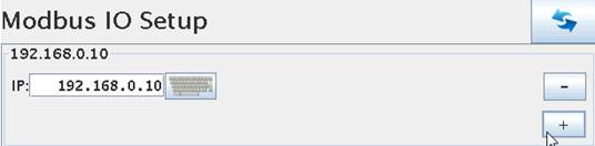
Press the “+”
sign just below the “-“ sign and in same row as the IP address we are defining.
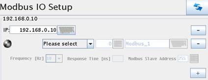
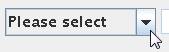
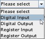
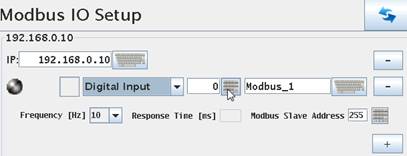
Define the first entry as an Input. Press the Keyboard sign
in the middle.
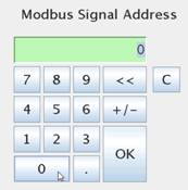
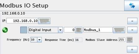
Define the first
Modbus signal address as “0” which is the local address on the Modbus node for
input 0 (first input on Modbus node).
This will
activate the Modbus node and a Green light will appear. In this case the Input
is high – indicated by the dark grey box next to the green light.
Each Individual Input and output has to be
defined in this manner.
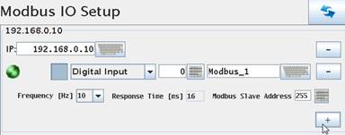
Press on the “+”
sign below the previous Modbus definition to define the next Input.
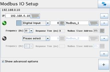
Define this next Input like the previous one,
but this one has the next local address which is “1”.
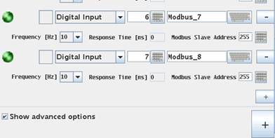
In this case the Modbus node has 8 inputs and
therefore address 0 to 7 has been defined.
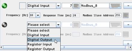
After all the Inputs has been defined – then
define the Outputs in similar way.
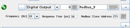
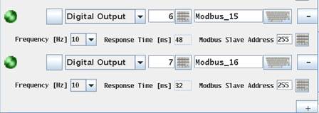
Continue until all 8 Outputs have been defined
(local address 0 – 7).
In case of more than 8 in and 8 outputs the Modbus
“scan” frequency maybe has to be reduced.
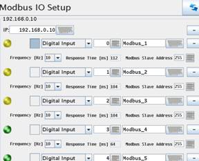
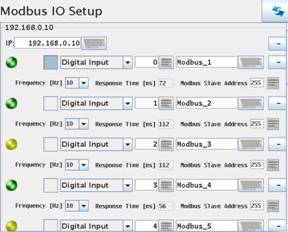
If there is
yellow light in some Modbus nodes representation in the UR robot menu (not on
the node) then the frequency has to be reduced until all in/output is green - properly
5 Hz is recommended.
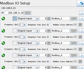
Make sure there is no more flickering yellow
light and all is green which indicates that the Scan frequency is correct.
Press the I/O tab
and notice that there is now a Tab called the Modbus.

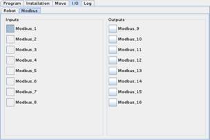
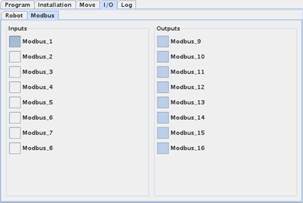
This screen shows the status of the Modbus
Inputs and Outputs and the Outputs can be manipulated. On the right side all
outputs has been set high.
The Modbus Inputs and Outputs are no available
to be used in the program structure.
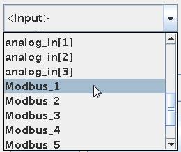
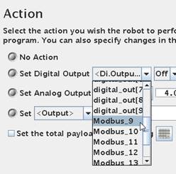
Modbus Inputs
ready to be used. Modbus
Outputs ready to be used.
When programming the robot you might
experience sometime the robot is stopping with a safety stop called “Joint
Limit Violation” or similar error messages. And you can observe the robot was
trying to reach a Waypoint you had set, but it was not possible due to
mathematically and physical limitations. This can especially happen in MoveL
(linear mode) programming. It does not mean that the robot cannot go to the
Waypoint you have defined, but it cannot reach there in the way programmed.
Consider you arm and reaching for a coin that
is in between your elbow and wrist. If you are not allowed to move you body posture
– then it is very difficult to reach and grab the coin. But when you can move
you body posture then it is very easy to pick the coin.
Similar situation can occur during programming
the robot where it will be impossible for the robot to take a linear move from
where it was to reach and grab the coin. The robot will attempt and you will se
a rapid increase in speed and very fast thereafter the robot stop with joint
error messages in order not to spoil the robot.
Just reposition the robot posture and
waypoints and the robot can reach the target.


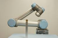
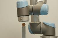
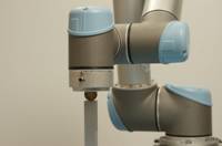
The UR robot is equipped with a Safety stop
when the robot meets a force that is 150 Newton (approximate 15 Kg).
Since there is a safety margin the value is
actually lower than 150 Newton in order to ensure that the robot complies with
this ISO standard.
On the other hand
the robot has a lifting capacity of 5 Kg (approximate 50 Newton) so the safety
stops cannot be lower than 50 Newton. So the actual value is between 50 Newton
and 150 Newton.
This You tube
video shows how the light guard can be applied.
http://www.youtube.com/watch?v=U6_Hk9v-XSs
Note that when
the person enters through the light guard – the robot stops. Only when the person
leaves the area and press the reset button which is outside the area – the
robot continues from the position it stopped.
Please note that the Green and Red light you
see at the reset button are controlled by the relay on the light guard – i.e.
not by the robot.
When the light guard output is high a relay is
activated and when the output is low the relay is deactivated and the contact
associated with the relay controls the red and green light.
When connecting an external Emergency Stop or
interconnects the Emergency Stop circuit with another machine there is something
about potential free connections we need to consider.
In this example we consider a CNC machine as
the “other” machine to interconnect the Robot Emergency circuit with. We actually don’t want to mix the power
voltage on the CNC with the Power voltage on the robot - nor do we want to mix
the GND on the two machines. Because if we mix the Power voltages on the
machines - the internal Power supplies could start fighting and there could be
a risk of damage if there for some reason was a difference in the voltage
levels. So in a case where there is 12 Volt DC on one machine and 24 Volt DC on
the other machine is a good example where we do not want to mix such power
levels because then we could damage the electronic circuits - and then it is
good we have a method to overcome that.
Another fundamental thing that is important to
know is that we normally say that Emergency stop is to protect humans from
danger - so when we see a danger we can press an Emergency stop and the machine
stops.
And the Safety stop (as explained in previous
chapter) is a controlled method to protect the machine and humans form a
potential damage.
This fact is very important to remember when
we are working with these two different safety functions and why there are
different level of severity to these circuits - because we can easy understand
that the Emergency Stop circuit has the highest and most severe rules to comply
to because it deals with protection of humans.
However the basic of the circuits and how they
work are very similar principle which is the principle of Serial connection of
switches that all have to be closed to have a normal operational condition. As
soon as the loop i.e. the Serial connection is open at any place - the Safety
circuit detects that and we activate the Emergency Stop or Safety stop.
Next important thing to know is that Emergency
stop circuit has to be hardwired i.e. it cannot be programmed - for example
sending a Emergency stop switch to a PLC input and then the PLC program perform
the Emergency Stop routine - this is not allowed because then there would be
two main risk - either the risk that the programmer made an error so the program
does not detects the input change - or there is the possibility of a PLC error
and if someone presses the Emergency Stop, but the PLC is in error then the
Emergency stop routine will not happen - this is not good. Therefore Emergency stop circuits has to be
made of approved and certified components the comply with the highest class
(standard) of safety. This means it is not good to insert or make to much
modification to emergency stop circuit - unless we use approved equipment -
that is Emergency Stop relays. Such functionality is often build into nowadays
standard machines.
Also what is important to understand is that
when talking about Emergency Stop circuits we normally has two loops for the
highest class of safety - the reason for that is to be sure to detect an
Emergency stop situation even if there is error on the equipment. Consider a
contact set is hanging inside the Emergency stop pushbutton - and when someone
press the contact still hangs - and no Emergency Stop is detected - that’s not
good - so instead there must be two contact set in a good Emergency Stop
circuit for each pushbutton because if one contact is hanging - then the other
contact will properly still work when someone press and the Emergency stop is
detected.
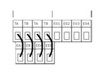
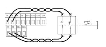
Remember that we need two loops - so that’s why you see two sets of TA - EA,
TB - EB and TA - EEA, TB – EEB inside the robot cabinet.
On the top left figure you see the External
Emergency Stop “jumped out” i.e. there is no External Emergency stop used
(That’s how the robot is configured as standard) - only the internal Emergency
stop is active (the one on the display) which is wired internally in the
Robot).
TA feeds EA and TB feeds EB and the same on
the second set of TA - EEA, TB - EEB. (EA-EB and EEA-EEB are Emergency Stop
approved inputs) and at any place this serial connection is open - we detect an
Emergency Stop. So actually what you see is that TA-EA and TB-EB is logical
short circuit because of the red wires mounted and same goes with TA-EEA and
TB-EEB. That’s what the internal circuit likes when there is no Emergency Stop
- as soon TA-EA or TB-EB or TA-EEA or TB-EEB is no longer logical short circuit
- we detect an Emergency Stop. Any of the four open will trigger an Emergency
stop.
On the top right figure you see a
configuration of an external push button applied. This is an extra Emergency
Stop Push button (not the one on the CNC machine) in case you would like to
have an Emergency Stop push button somewhere else than on the Robot Monitor.
Notice how there is two sets of contacts according to highest Class of safety -
and if just one of the contacts open - we detect an Emergency Stop - and the
robot Stops.
Please note that you still need the jumper
TA-EEA and TB-EEB (not show on the drawing) – otherwise there would be an
Emergency Stop triggered.
One important
thing to be aware of is that if TA-EA or TB-EB is open – then the internal
Emergency Stop relay is open i.e. E01-E02 and E03-E04 contacts opens. Whereas
if TA-EEA or TB-EEB is open - then the internal Emergency Stop relay is not
open i.e. E01-E02 and E03-E04 is still closed.
(This is useful
later when we connect to another machine).

This figure shows an example how two machines
can be connected together - and this is what we need in this case. The example
speaks about two Robots connected - which are also possible, but in our case we
have one CNC machine (A) and one Robot (B) to connect, but it is still the same
principle.
So far you can see the terminals E01, E02, E03
and E04 have not been used, but we are going to use those now. This is just two
contact sets E01-E02 is one contact and E03-E04 is another contact set. These
contact sets are normally closed - and both contact sets also opens when there
is an Emergency Stop condition. This is great and we can use that to tell
another machine that there is an Emergency stop on the Machine which is holding
this contact set.

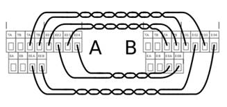
Consider that we have both an External
Emergency Push Button (left figure) and we also have a interconnection with
another machine (right figure).
Remember that TA-EA and TB-EB and TA-EEA and
TB-EEB need to be short circuit to have a normal condition without Emergency
Stop. So follow the wire from TA on machine "A" down to “first
contact set” of external Emergency Stop and back to EA.
Same - follow the wire from TB on machine “A”
down to “second contact set” of external Emergency Stop and back to EB (The two
loops are closed).
Now follow the wire from TA on machine “A”
over to E03 on machine “B” through a closed contact to E04 and back to EEA on
machine “A”.
Same – follow the wire from TB on machine “A”
over to E01 on machine “B” through a closed contact to E02 and back to EEB on
machine “A”. The two loops are closed.
The same principle for machine “B” over to
machine “A”.
Now consider an Emergency Stop on machine “A”
or a External Emergency Stop on machine “A” – first of all it stops machine “A”
– and because the internal Emergency Stop relay on machine “A” opens up E01-E02
and E03-E04 - it breaks the loop of
TA-EEA and TB-EEB on machine “B” – so machine “B” also stops.
Now – because we used TA-EEA and TB-EEB as the
loop to break on machine “B” – it causes the machine “B” to stop OK, but the
internal Emergency relay on machine “B” does not open E01-E02 and E03-E04 on
machine "B". That very good because now we can reset the Emergency
Stop on “A” – which closes E01-E02 and E03-E04 on machine “A” - which cause the
loop TA-EEA and TB-EEB on machine “B” to close – and both machines can restart.
(Note: If the
Emergency stop relay had opened on the machine "B" - which is the
machine without the real Emergency Stop pressed – then we would not have been
able to reset again – because both machines would held each other “open”, but
now we can).
It is possible to have almost as many extra
Emergency Stop as you want (only limit is the resistance in the wire and
contacts.